We’ve seen that CNNs can learn the content of an image for classification purposes, but what else can they do? This tutorial will look at the Generative Adversarial Network (GAN) which is able to learn from a set of images and create an entirely new ‘fake’ image which isn’t in the training set. Why? By the end of this tutorial you’ll get know why this might be done and how to do it.
Introduction
Generative Adversarial Networks (GANs) were proposed by Ian Goodfellow et al in 2014 at annual the Neural Information and Processing Systems (NIPS) conference. The original paper is available on Arxiv along with a later tutorial by Goodfellow delivered at NIPS in 2016 here. I’ve read both of these (and others) as well as taking a look at other tutorials but sometimes things just weren’t clear enough for me. This blog from B. Amos has been helpful in getting my thoughts organised on this series, and hopefully I can build on this a little and make things more concrete.
What's a GAN?
GANs are used in a number of ways, for example:
- to generate new images based upon some training data. For our tutorial, we will train with a database of faces and ask the network to produce a new face.
- to do ‘inpainting’ or ‘image completion’. This is where part of a scene may be missing and we wish to recover the full image. It could be that we want to remove parts of the image e.g. people, and fill-in the background.
There are two components in a GAN which try to work against each other (hence the ‘adversarial’ part).
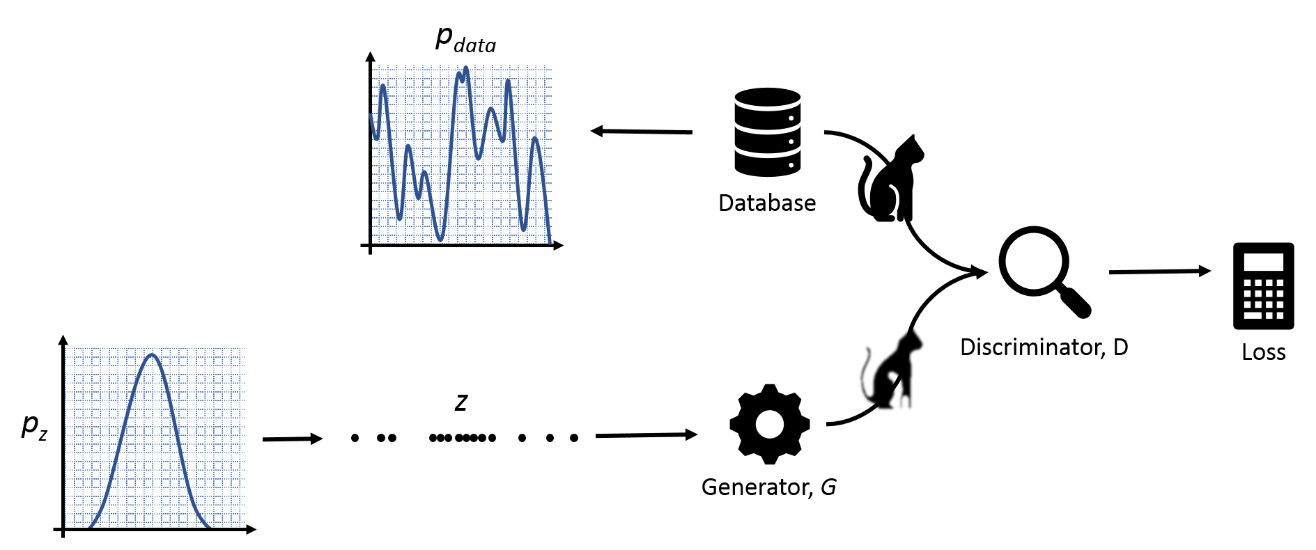
- The Generator (G) starts off by creating a very noisy image based upon some random input data. Its job is to try to come up with images that are as real as possible.
- The Discriminator (D) is trying to determine whether an image is real or fake.
Though these two are the primary components of the network, we also need to write some functions for importing data and dealing with the training of this two-stage network. Part 1 of this tutorial will go through some background and mathematics, in Part 2 we will do some general housekeeping and get us prepared to write the main model of our network in Part 3.
Background
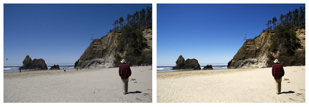
There are a number of situations where you may want to use a GAN. A common task is for image completion or ‘in-painting’. This would be where we have an image and would like to remove some obstruction or imperfection by replacing it with the background. Maybe there’s a lovely holiday photo of beautiful scenery, but there are some people you don’t know spoiling the view. Figure 1 shows an example of the result of image completion using PhotoShop on such an image.

We have a couple of options if we want to try and do this kind of image completion ourselves. Let’s say we draw around an area we want to change:
- If we’ve never seen a beach or the sky before, well we may just have to use the neighbouring pixels to inform our in-filling. If we’re feeling fancy, we would look a little further afield and use that information too ( i.e. is there just sky around the area, or is there something else).
- Or… we could look at the image as a whole and try to see what would fit best. For this we would have to use our knowledge of similar scenes we’ve observed.
This is the difference between using (1) contextual and (2) perceptual information. But before we look more heavily into this, let’s take a look at the idea behind a GAN.
Generative Adversarial Networks
We’ve said that there are two components in a GAN, the generator and the discriminator. Here, we’ll look more closely at what they do.
Our purpose is to create images which are as realistic as possible. So much so, that they are able to fool not only humans, but the computer that has generated them. You will often see GANs being compared to money counterfeiting: our generator is trying to create fake money whilst our discriminator is trying to tell the difference between the real and fake bills. How does this work?
Say we have an image $x$ which our discriminator $D$ is analysing. $D(x)$ gives a low value near to 0 if the image looks normal or ‘natural’ and a higher value near to 1 if it thinks the image is fake - this could mean it is very noisy for example. The generator $G$ takes a vector $z$ that has been randomly sampled from a very simple, but well known, distribution e.g. a uniform or normal distribution. The image that is produced by $G(z)$ should help to train the function at $D$. We alternate showing the discriminator a real image (which will change its parameters to give a low output) and then an image from $G$ (which will change $D$ to give a higher output). At the same time, we want $G$ to also be learning to produce more realistic images which are more likely to fool $D$. We want $G$ to minimise the output of $D$ whilst $D$ is trying to maximise the same thing. They are playing a ‘minimax’ game against each other, which is where we get the term ‘adversarial’ training.

Let’s keep going with the maths…
This kind of network has a lot of latent (hidden) variables that need to be found. But we can start from a strong position by using a distribution that we know very well like a uniform distribution.
- The known distribution we denote $p_z$ We will randomly draw a vector $z$ from $p_z$.
- We know that our data must have some distribution but we do not know this. We’ll call this $p_{data}$
- Our generator will try to learn its own distribution $p_g$. Our goal is for $p_g = p_{data}$
We have two networks to train, $D$ and $G$:
- We want to minimise $D(x)$ if $x$ is drawn from our true distribution $p_{data}$ i.e. minimise $D(x)$ if it’s not.
- and maximise $D(G(z))$ i.e. minimise $1 - D(G(z))$.
More formally:
Where $\mathbb{E}$ is the expectation. The advantage of working with neural networks is that we can easily compute gradients and use backpropagation to perform training. This is because the generator and the discriminator are defined by the multi-layer perceptron (MLP) parameters $\theta_g$ and $\theta_d$ respectively.
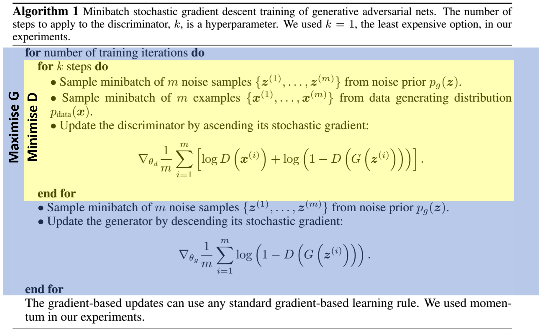
We will train the networks (the $G$ and the $D$) one at a time, fixing the weights of one whilst training the other. From the GAN paper by Goodfellow et al we get the pseudo code for this procedure:

Notice that with $k=1$ we are training $D$ then $G$ one after the other. What is the training actually doing? Fig. 4 shows the distribution $p_g$ of the generator in green. Notice that with each training step, the $p_g$ becomes more like the true distribution of the image data $p_{data}$ in black. After each alternation, the error is backpropagated to udate the weights on the network that is not being held fixed. The discriminator eventually reaches its lowest maximum where it is no longer able to tell the difference between the true and fake images.

What's Next?"
That really is it. The basics of a GAN are just a game between two networks, the generator $G$, which produces images from some latent variables $z$, and the discriminator $D$ which tries to detect the faked images.
Implementing this in Python seems old-hat to many and there are many pre-built solutions available. The work in this tutorial series will mostly follow the base-code from carpedm20’s DCGAN-tensorflow repository.
In the next post, we’ll get ourselves organised, make sure we have some dependencies, create some files and get our training data sorted.
As always, if there’s anything wrong or that doesn’t make send please get in contact and let me know. A comment here is great.
comments powered by Disqus


