
One of the greatest limiting factors for training effective deep learning frameworks is the availability, quality and organisation of the training data. To be good at classification tasks, we need to show our CNNs etc. as many examples as we possibly can. However, this is not always possible especially in situations where the training data is hard to collect e.g. medical image data. In this post, we will learn how to apply data augmentation strategies to n-Dimensional images get the most of our limited number of examples.
Introduction
If we take any image, like our little Android below, and we shift all of the data in the image to the right by a single pixel, you may struggle to see any difference visually. However, numerically, this may as well be a completely different image! Imagine taking a stack of 10 of these images, each shifted by a single pixel compared to the previous one. Now consider the pixels in the images at [20, 25] or some arbitrary location. Focusing on that point, each pixel has a different colour, different average surrounding intensity etc. A CNN take these values into account when performing convolutions and deciding upon weights. If we supplied this set of 10 images to a CNN, it would effectively be making it learn that it should be invariant to these kinds of translations.

Android

Shifted 1 pixel right

Shifted 10 pixels right
Of course, translations are not the only way in which an image can change, but still visually be the same image. Consider rotating the image by even a single degree, or 5 degrees. It’s still an Android. Traning a CNN without including translated and rotated versions of the image may cause the CNN to overfit and assume that all images of Androids have to be perfectly upright and centered.
Providing deep learning frameworks with images that are translated, rotated, scaling, intensified and flipped is what we mean when we talk about data augmentation.
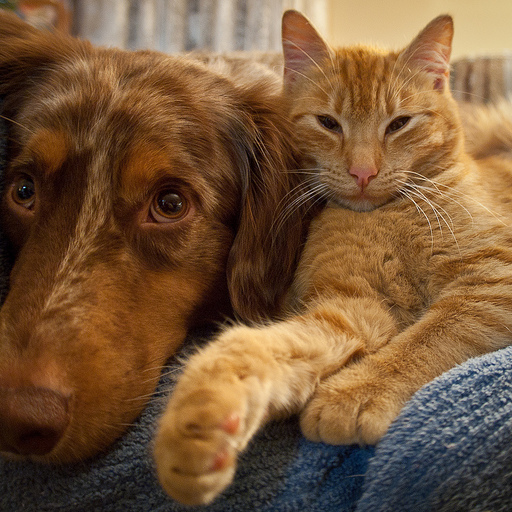
In this post we’ll look at how to apply these transformations to an image, even in 3D and see how it affects the performance of a deep learning framework. We will use an image from flickr user andy_emcee as an example of a 2D nautral image. As this is an RGB (color) image it has shape [512, 640, 3], one layer for each colour channel. We could take one layer to make this grayscale and truly 2D, but most images we deal with will be color so let’s leave it. For 3D we will use a 3D MRI scan
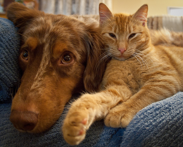
RGB Image shape=[512, 640, 3]
Augmentations
As usual, we are going to write our augmentation functions in python. We’ll just be using simple functions from numpy and scipy.
Translation
In our functions, image is a 2 or 3D array - if it’s a 3D array, we need to be careful about specifying our translation directions in the argument called offset. We don’t really want to move images in the z direction for a couple of reasons: firstly, if it’s a 2D image, the third dimension will be the colour channel, if we move the image through this dimension the image will either become all red, all blue or all black if we move it -2, 2 or greater than these respectively; second, in a full 3D image, the third dimension is often the smallest e.g. most medical scans. In our translation function below, the offset is given as a length 2 array defining the shift in the y and x directions respectively (dont forget index 0 is which horizontal row we’re at in python). We hard-code z-direction to 0 but you’re welcome to change this if your use-case demands it. To ensure we get integer-pixel shifts, we enforce type int too.
def translateit(image, offset, isseg=False):
    order = 0 if isseg == True else 5

    return scipy.ndimage.interpolation.shift(image, (int(offset[0]), int(offset[1]), 0), order=order, mode='nearest')
Here we have also provided the option for what kind of interpolation we want to perform: order = 0 means to just use the nearest-neighbour pixel intensity and order = 5 means to perform bspline interpolation with order 5 (taking into account many pixels around the target). This is triggered with a Boolean argument to the scaleit function called isseg so named because when dealing with image-segmentations, we want to keep their integer class numbers and not get a result which is a float with a value between two classes. This is not a problem with the actual image as we want to retain as much visual smoothness as possible (though there is an arugment that we’re introducing data which didn’t exist in the original image). Similarly, when we move our image, we will leave a gap around the edges from which it’s moved. We need a way to fill in this gap: by default shift will use a contant value set to 0. This may not be helpful in some case, so it’s best to set the mode to 'nearest' which takes the cloest pixel-value and replicates it. It’s barely noticable with small shifts but looks wrong at larger offsets. We need to be careful and only apply small translations to our data.

Original Image
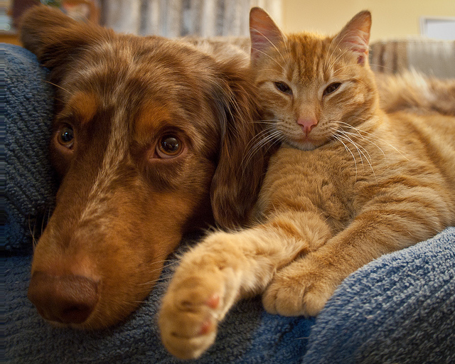
Shifted 5 pixels right
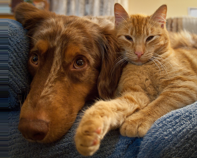
Shifted 25 pixels right
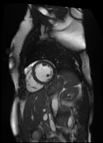

Original Image and Segmentation
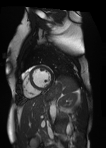
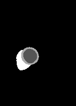
Shifted [-3, 1] pixels
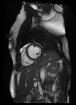
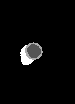
Shifted [4, -5] pixels
Scaling
When scaling an image, i.e. zooming in and out, we want to increase or decrease the area our image takes up whilst keeping the image dimensions the same. We scale our image by a certain factor. A factor > 1.0 means the image scales-up, and factor < 1.0 scales the image down. Note that we should provide a factor for each dimension: if we want to keep the same number of layers or slices in our image, we should set last value to 1.0. To determine the intensity of the resulting image at each pixel, we are taking the lattice (grid) on which each pixel sits and using this to perform interpolation of the surrounding pixel intensities. scipy provides a handy function for this called zoom:
The definition is probably more complex than one would think:
def scaleit(image, factor, isseg=False):
    order = 0 if isseg == True else 3

    height, width, depth= image.shape
    zheight             = int(np.round(factor * height))
    zwidth              = int(np.round(factor * width))
    zdepth              = depth

    if factor < 1.0:
        newimg  = np.zeros_like(image)
        row     = (height - zheight) // 2
        col     = (width - zwidth) // 2
        layer   = (depth - zdepth) // 2
        newimg[row:row+zheight, col:col+zwidth, layer:layer+zdepth] = interpolation.zoom(image, (float(factor), float(factor), 1.0), order=order, mode='nearest')[0:zheight, 0:zwidth, 0:zdepth]

        return newimg

    elif factor > 1.0:
        row     = (zheight - height) // 2
        col     = (zwidth - width) // 2
        layer   = (zdepth - depth) // 2

        newimg = interpolation.zoom(image[row:row+zheight, col:col+zwidth, layer:layer+zdepth], (float(factor), float(factor), 1.0), order=order, mode='nearest')

        extrah = (newimg.shape[0] - height) // 2
        extraw = (newimg.shape[1] - width) // 2
        extrad = (newimg.shape[2] - depth) // 2
        newimg = newimg[extrah:extrah+height, extraw:extraw+width, extrad:extrad+depth]

        return newimg

    else:
        return image
There are three possibilities that we need to consider - we are scaling up, down or no scaling. In each case, we want to return an array that is equal in size to the input image. For the scaling down case, this involves making a blank image the same shape as the input, and finding the corresponding box in the resulting scaled image. For scaling up, it’s unnecessary to perform the scaling on the whole image, just the portion that will be ‘zoomed’ - so we pass only part of the array to the zoom function. There may also be some error in the final shape due to rounding, so we do some trimming of the extra rows and colums before passing it back. When no scaling is done, we just return the original image.

Original Image
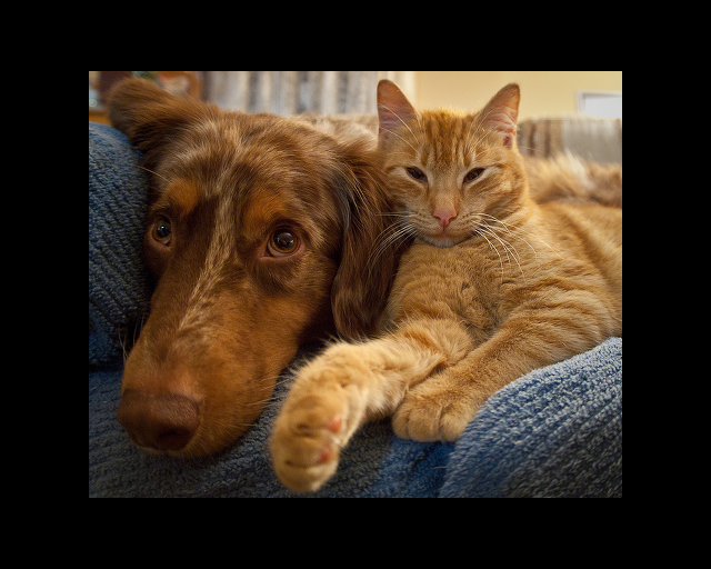
Scale-factor 0.75
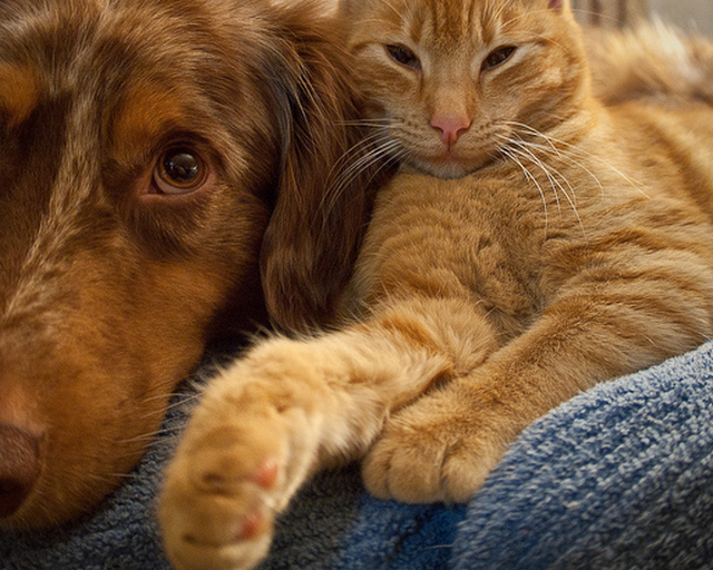
Scale-factor 1.25


Original Image and Segmentation
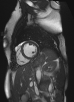
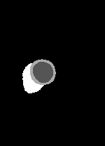
Scale-factor 1.07
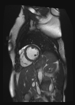
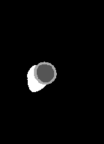
Scale-factor 0.95
Resampling
It may be the case that we want to change the dimensions of our image such that they fit nicely into the input of our CNN. For example, most images and photographs have one dimension larger than the other or may be of different resolutions. This may not be the case in our training set, but most CNNs prefer to have inputs that are square and of identical sizes. We can use the same scipy function interpolation.zoom to do this:
def resampleit(image, dims, isseg=False):
    order = 0 if isseg == True else 5

    image = interpolation.zoom(image, np.array(dims)/np.array(image.shape, dtype=np.float32), order=order, mode='nearest')

    if image.shape[-1] == 3: #rgb image
        return image
    else:
        return image if isseg else (image-image.min())/(image.max()-image.min())
The key part here is that we’ve replaced the factor argument with dims of type list. dims should have length equal to the number of dimensions of our image i.e. 2 or 3. We are calculating the factor that each dimension needs to change by in order to change the image to the target dims. We’ve forced the denominator of the scaling factor to be of type float so that the resulting factor is also float.
In this step, we are also changing the intensities of the image to use the full range from 0.0 to 1.0. This ensures that all of our image intensities fall over the same range - one fewer thing for the network to be biased against. Again, note that we don’t want to do this for our segmentations as the pixel ‘intensities’ are actually labels. We could do this in a separate function, but I want this to happen to all of my images at this point. There’s no difference to the visual display of the images because they are automaticallys rescaled to use the full range of display colours.
Rotation
This function utilises another scipy function called rotate. It takes a float for the theta argument which specifies the number of degrees of the roation (negative numbers rotate anti-clockwise). We want the returned image to be of the same shape as the input image so reshape = False is used. Again we need to specify the order of the interpolation on the new lattice. The rotate function handles 3D images by rotating each slice by the same theta.
def rotateit(image, theta, isseg=False):
    order = 0 if isseg == True else 5

    return rotate(image, float(theta), reshape=False, order=order, mode='nearest')

Original Image
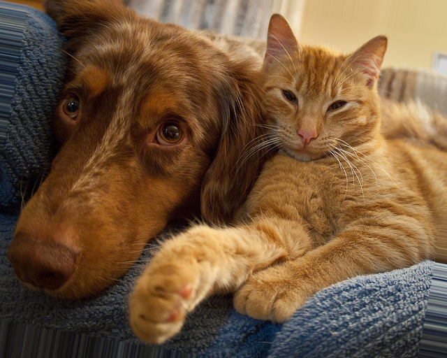
Theta = -10.0
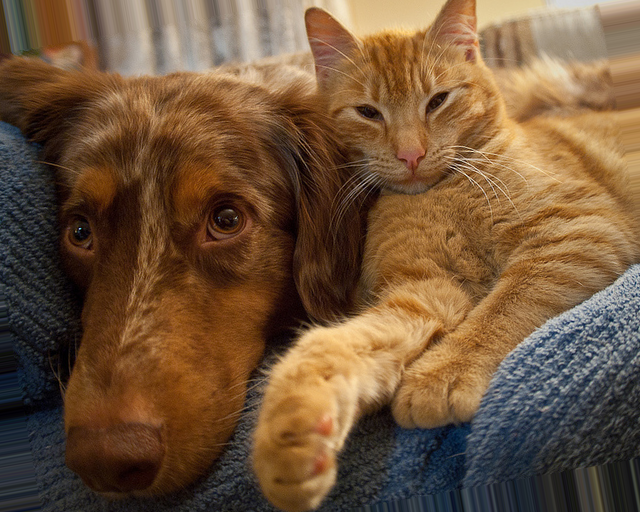
Theta = 10.0


Original Image and Segmentation
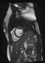
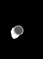
Theta = 6.18
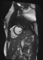
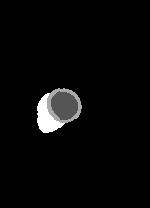
Theta = -1.91
Intensity Changes
The final augmentation we can perform is a scaling in the intensity of the pixels. This effectively brightens or dims the image by appling a blanket increase or decrease across all pixels. We specify the amount by a factor: factor < 1.0 will dim the image, and factor > 1.0 will brighten it. Note that we don’t want a factor = 0.0 as this will blank the image.
def intensifyit(image, factor):

    return image*float(factor)
Flipping
One of the most common image augmentation procedures for natural images (dogs, cats, landscapes etc.) is to do flipping. The premise being that a dog is a dog no matter which was it’s facing. Or it doesn’t matter if a tree is on the right or the left of an image, it’s still a tree.
We can do horizontal flipping, left-to-right or vertical flipping, up and down. It may make sense to do only one of these (if we know that dogs don’t walk on their heads for example). In this case, we can specify a list of 2 boolean values: if each is 1 then both flips are performed. We use the numpy functions fliplr and flipup for these.
As with resampling, the intensity changes are modified to take the range of the display so there wont be a noticable difference in the images. The maximum value for display is 255 so increasing this will just scale it back down.
def flipit(image, axes):

    if axes[0]:
        image = np.fliplr(image)
    if axes[1]:
        image = np.flipud(image)

    return image
Cropping
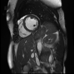
This may be a very niche function, but it’s important in my case. Often in natrual image processing, random crops are done on the image in order to give patches - these patches often contain most of the image data e.g. 224 x 224 patch rather than 299 x 299 image. This is just another way of showing the network a very similar but also entirely different image. Central crops are also done. What’s different in my case is that I always want my segmentation to be fully-visible in the image that I show to the network (I’m working with 3D cardiac MRI segmentations).
So this function looks at the segmentation and creates a bounding box using the outermost pixels. We’re producing ‘square’ crops with side-length equal to the width of the image (the shortest side not including the depth). In this case, the bounding box is created and, if necessary, the window is moved up and down the image to make sure the full segmentation is visible. It also makes sure that the output is always square in the case that the bounding box moves off the image array.
def cropit(image, seg=None, margin=5):

    fixedaxes = np.argmin(image.shape[:2])
    trimaxes  = 0 if fixedaxes == 1 else 1
    trim    = image.shape[fixedaxes]
    center  = image.shape[trimaxes] // 2

    print image.shape
    print fixedaxes
    print trimaxes
    print trim
    print center

    if seg is not None:

        hits = np.where(seg!=0)
        mins = np.argmin(hits, axis=1)
        maxs = np.argmax(hits, axis=1)

        if center - (trim // 2) > mins[0]:
            while center - (trim // 2) > mins[0]:
                center = center - 1
            center = center + margin

        if center + (trim // 2) < maxs[0]:
            while center + (trim // 2) < maxs[0]:
                center = center + 1
            center = center + margin

    top    = max(0, center - (trim //2))
    bottom = trim if top == 0 else center + (trim//2)

    if bottom > image.shape[trimaxes]:
        bottom = image.shape[trimaxes]
        top = image.shape[trimaxes] - trim

    if trimaxes == 0:
        image   = image[top: bottom, :, :]
    else:
        image   = image[:, top: bottom, :]

    if seg is not None:
        if trimaxes == 0:
            seg   = seg[top: bottom, :, :]
        else:
            seg   = seg[:, top: bottom, :]

        return image, seg
    else:
        return image
Note that this function will work to square an image even when there is no segmentation given. We also have to be careful about which axes we take as the ‘fixed’ length for the square and which one to trim.

Original Image
Cropped


Original Image and Segmentation
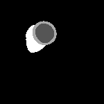
Cropped
Application
We should be careful about how we apply our transformations. For example, if we apply multiple transformations to the same image we need to make sure that we don’t apply ‘resampling’ after ‘intensity changes’ because this will reset the range of the image, defeating the point of the intensification. However, as we will generally want our data to span the same range, wholesale intensity shifts are less often seen. We also want to make sure that we are not being over zealous with the augmentations either - we need to set limits for our factors and other arguments.
When I implement data augmentation, I put all of these transforms into one script which can be downloaded here: transforms.py. I then call the transforms that I want from another script.
We create a set of cases, one for each transformation, which draws random (but controlled) parameters for our augmentations, remember we don’t want anything too extreme. We don’t want to apply all of these transformations every time, so we also create an array of random length (number of transformations) and randomly assigned elements (the transformations to apply).
np.random.seed()
numTrans     = np.random.randint(1, 6, size=1)
allowedTrans = [0, 1, 2, 3, 4]
whichTrans   = np.random.choice(allowedTrans, numTrans, replace=False)
We assign a new random.seed every time to ensure that each pass is different to the last. There are 5 possible transformations so numTrans is a single random integer between 1 and 5. We then take a random.choice of the allowedTrans up to numTrans. We don’t want to apply the same transformation more than once, so replace=False.
After some trial and error, I’ve found that the following parameters are good:
- rotations -
theta$ \in [-10.0, 10.0] $ degrees - scaling -
factor$ \in [0.9, 1.1] $ i.e. 10% zoom-in or zoom-out - intensity -
factor$ \in [0.8, 1.2] $ i.e. 20% increase or decrease - translation -
offset$ \in [-5, 5] $ pixels - margin - I tend to set at either 5 or 10 pixels.
For an image called thisim and segmentation called thisseg, the cases I use are:
if 0 in whichTrans:
    theta   = float(np.around(np.random.uniform(-10.0,10.0, size=1), 2))
    thisim  = rotateit(thisim, theta)
    thisseg = rotateit(thisseg, theta, isseg=True) if withseg else np.zeros_like(thisim)

if 1 in whichTrans:
    scalefactor  = float(np.around(np.random.uniform(0.9, 1.1, size=1), 2))
    thisim  = scaleit(thisim, scalefactor)
    thisseg = scaleit(thisseg, scalefactor, isseg=True) if withseg else np.zeros_like(thisim)

if 2 in whichTrans:
    factor  = float(np.around(np.random.uniform(0.8, 1.2, size=1), 2))
    thisim  = intensifyit(thisim, factor)
    #no intensity change on segmentation

if 3 in whichTrans:
    axes    = list(np.random.choice(2, 1, replace=True))
    thisim  = flipit(thisim, axes+[0])
    thisseg = flipit(thisseg, axes+[0]) if withseg else np.zeros_like(thisim)

if 4 in whichTrans:
    offset  = list(np.random.randint(-5,5, size=2))
    currseg = thisseg
    thisim  = translateit(thisim, offset)
    thisseg = translateit(thisseg, offset, isseg=True) if withseg else np.zeros_like(thisim)
In each case, a random set of parameters is found and passed to the transform functions. The image and segmentation are passed separately to each one. In my case, I only choose to flip horizontally by randomly choosing 0 or 1 and appending [0] such that the transform ignores the second axis. We’ve also added a boolean variable called withseg. When True the segmentation is augmented, otherwise a blank image is returned.
Finally, we crop the image to make it square before resampling it to the desired dims.
thisim, thisseg = cropit(thisim, thisseg)
thisim          = resampleit(thisim, dims)
thisseg         = resampleit(thisseg, dims, isseg=True) if withseg else np.zeros_like(thisim)
Putting this together in a script makes testing the augmenter easier: you can download the script here. Some things in the code to note:
- The script takes one mandatory argument (image filename) and an optional segmentation filename
- There’s a bit of error checking - are the files able to be loaded? Is it an rgb or full 3D image (3rd dimension greater than 3).
- We specify the final image dimensions, [224, 224, 8] in this case
- We also declare some default values for the parameters so that we can…
- …print out the applied transformations and their parameters at the end
- There’s a definition for a
plotitfunction that just creates a 2 x 2 matrix where the top 2 images are the originals and the bottom two are the augmented images. - There’s a commented out part which is what I used to save the images created in this post
In a live setting where we want to do data-augmentation on the fly, we would essentially call this script with the filenames or image arrays to augment and create as many augmentations of the images as we wish. We’ll take a look at this as an example in the next post.
Edit: 15/05/2018
- Added a
sliceshiftfunction totransforms.py. This takes in a 3D image and randomly shifts afractionof the slices using ourtranslateitfunction (which I’ve also updated slightly). This allows us to simulate motion in medical images.


