
This series will give some background to CNNs, their architecture, coding and tuning. In particular, this tutorial covers some of the background to CNNs and Deep Learning. We won’t go over any coding in this session, but that will come in the next one. What’s the big deal about CNNs? What do they look like? Why do they work? Find out in this tutorial.
Introduction
A convolutional neural network (CNN) is very much related to the standard NN we’ve previously encountered. I found that when I searched for the link between the two, there seemed to be no natural progression from one to the other in terms of tutorials. It would seem that CNNs were developed in the late 1980s and then forgotten about due to the lack of processing power. In fact, it wasn’t until the advent of cheap, but powerful GPUs (graphics cards) that the research on CNNs and Deep Learning in general was given new life. Thus you’ll find an explosion of papers on CNNs in the last 3 or 4 years.
Nonetheless, the research that has been churned out is powerful. CNNs are used in so many applications now:
- Object recognition in images and videos (think image-search in Google, tagging friends faces in Facebook, adding filters in Snapchat and tracking movement in Kinect)
- Natural language processing (speech recognition in Google Assistant or Amazon’s Alexa)
- Playing games (the recent defeat of the world ‘Go’ champion by DeepMind at Google)
- Medical innovation (from drug discovery to prediction of disease)
Dispite the differences between these applications and the ever-increasing sophistication of CNNs, they all start out in the same way. Let’s take a look.
CNN or Deep Learning?
The "deep" part of deep learning comes in a couple of places: the number of layers and the number of features. Firstly, as one may expect, there are usually more layers in a deep learning framework than in your average multi-layer perceptron or standard neural network. We have some architectures that are 150 layers deep. Secondly, each layer of a CNN will learn multiple 'features' (multiple sets of weights) that connect it to the previous layer; so in this sense it's much deeper than a normal neural net too. In fact, some powerful neural networks, even CNNs, only consist of a few layers. So the 'deep' in DL acknowledges that each layer of the network learns multiple features. More on this later.
Often you may see a conflation of CNNs with DL, but the concept of DL comes some time before CNNs were first introduced. Connecting multiple neural networks together, altering the directionality of their weights and stacking such machines all gave rise to the increasing power and popularity of DL.
We won't delve too deeply into history or mathematics in this tutorial, but if you want to know the timeline of DL in more detail, I'd suggest the paper "On the Origin of Deep Learning" (Wang and Raj 2016) available here. It's a lengthy read - 72 pages including references - but shows the logic between progressive steps in DL.
As with the study of neural networks, the inspiration for CNNs came from nature: specifically, the visual cortex. It drew upon the idea that the neurons in the visual cortex focus upon different sized patches of an image getting different levels of information in different layers. If a computer could be programmed to work in this way, it may be able to mimic the image-recognition power of the brain. So how can this be done?
A CNN takes as input an array, or image (2D or 3D, grayscale or colour) and tries to learn the relationship between this image and some target data e.g. a classification. By ‘learn’ we are still talking about weights just like in a regular neural network. The difference in CNNs is that these weights connect small subsections of the input to each of the different neurons in the first layer. Fundamentally, there are multiple neurons in a single layer that each have their own weights to the same subsection of the input. These different sets of weights are called ‘kernels’.
It’s important at this stage to make sure we understand this weight or kernel business, because it’s the whole point of the ‘convolution’ bit of the CNN.
Convolution and Kernels
Convolution is something that should be taught in schools along with addition, and multiplication - it’s just another mathematical operation. Perhaps the reason it’s not, is because it’s a little more difficult to visualise.
Let’s say we have a pattern or a stamp that we want to repeat at regular intervals on a sheet of paper, a very convenient way to do this is to perform a convolution of the pattern with a regular grid on the paper. Think about hovering the stamp (or kernel) above the paper and moving it along a grid before pushing it into the page at each interval.
This idea of wanting to repeat a pattern (kernel) across some domain comes up a lot in the realm of signal processing and computer vision. In fact, if you’ve ever used a graphics package such as Photoshop, Inkscape or GIMP, you’ll have seen many kernels before. The list of ‘filters’ such as ‘blur’, ‘sharpen’ and ‘edge-detection’ are all done with a convolution of a kernel or filter with the image that you’re looking at.
For example, let’s find the outline (edges) of the image ‘A’.

A
We can use a kernel, or set of weights, like the ones below.
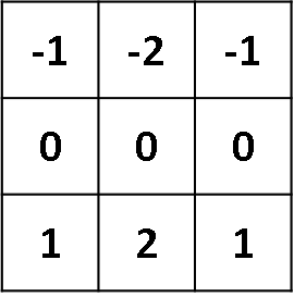
Finds horizontals
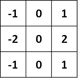
Finds verticals
A kernel is placed in the top-left corner of the image. The pixel values covered by the kernel are multiplied with the corresponing kernel values and the products are summated. The result is placed in the new image at the point corresponding to the centre of the kernel. An example for this first step is shown in the diagram below. This takes the vertical Sobel filter (used for edge-detection) and applies it to the pixels of the image.
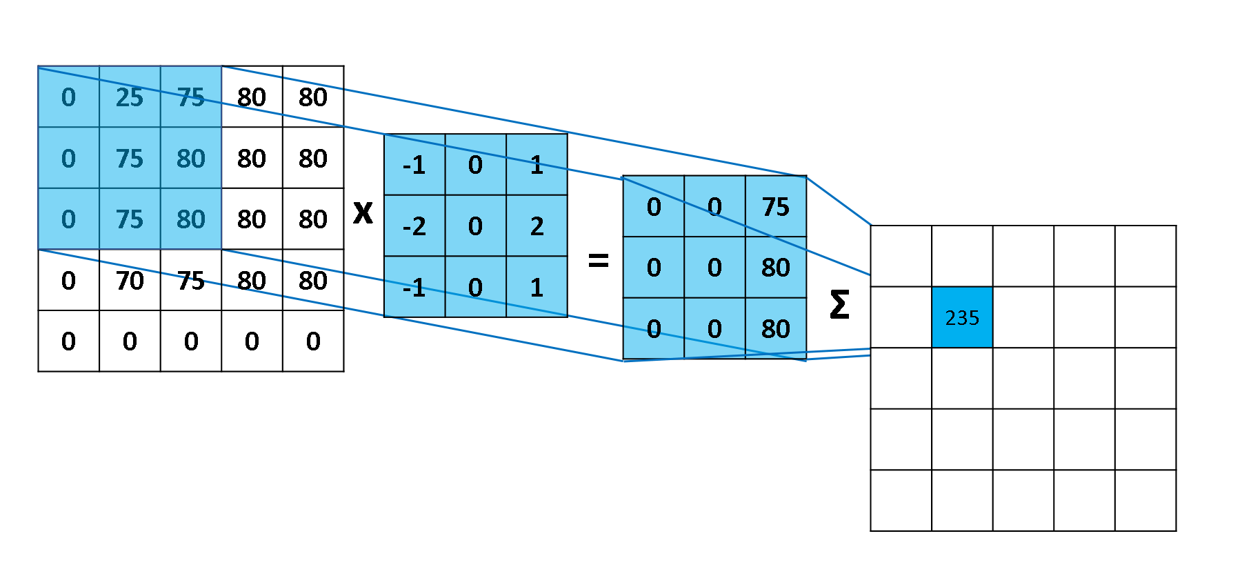
A step in the Convolution Process.
The kernel is moved over by one pixel and this process is repated until all of the possible locations in the image are filtered as below, this time for the horizontal Sobel filter. Notice that there is a border of empty values around the convolved image. This is because the result of convolution is placed at the centre of the kernel. To deal with this, a process called ‘padding’ or more commonly ‘zero-padding’ is used. This simply means that a border of zeros is placed around the original image to make it a pixel wider all around. The convolution is then done as normal, but the convolution result will now produce an image that is of equal size to the original.
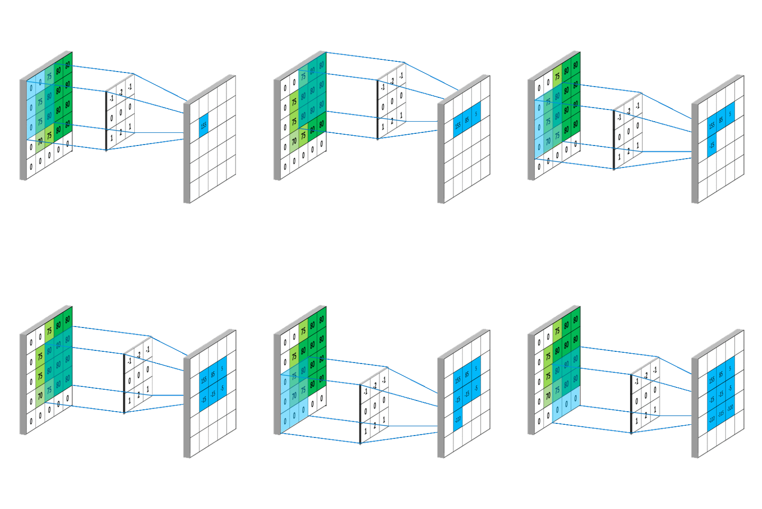
The kernel is moved over the image performing the convolution as it goes.
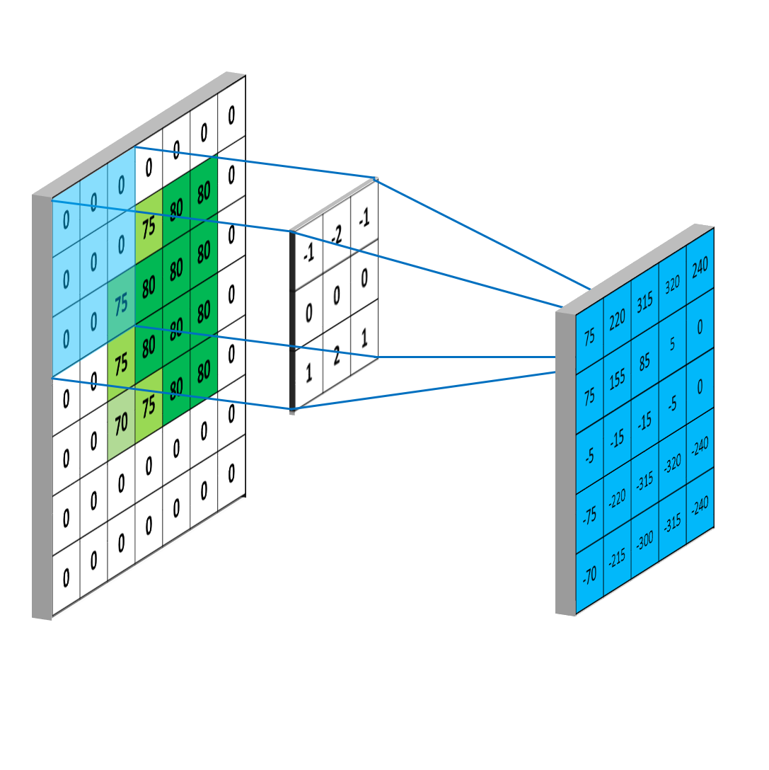
Zero-padding is used so that the resulting image doesn't shrink.
Now that we have our convolved image, we can use a colourmap to visualise the result. Here, I’ve just normalised the values between 0 and 255 so that I can apply a grayscale visualisation:

Result of the convolution
This dummy example could represent the very bottom left edge of the Android’s head and doesn’t really look like it’s detected anything. To see the proper effect, we need to scale this up so that we’re not looking at individual pixels. Performing the horizontal and vertical sobel filtering on the full 264 x 264 image gives:
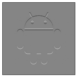
Horizontal Sobel
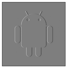
Vertical Sobel

Combined Sobel
Where we’ve also added together the result from both filters to get both the horizontal and vertical ones.
How does this feed into CNNs?
Clearly, convolution is powerful in finding the features of an image if we already know the right kernel to use. Kernel design is an artform and has been refined over the last few decades to do some pretty amazing things with images (just look at the huge list in your graphics software!). But the important question is, what if we don’t know the features we’re looking for? Or what if we do know, but we don’t know what the kernel should look like?
Well, first we should recognise that every pixel in an image is a feature and that means it represents an input node. The result from each convolution is placed into the next layer in a hidden node. Each feature or pixel of the convolved image is a node in the hidden layer.
We’ve already said that each of these numbers in the kernel is a weight, and that weight is the connection between the feature of the input image and the node of the hidden layer. The kernel is swept across the image and so there must be as many hidden nodes as there are input nodes (well actually slightly fewer as we should add zero-padding to the input image). This means that the hidden layer is also 2D like the input image. Sometimes, instead of moving the kernel over one pixel at a time, the stride, as it’s called, can be increased. This will result in fewer nodes or fewer pixels in the convolved image. Consider it like this:
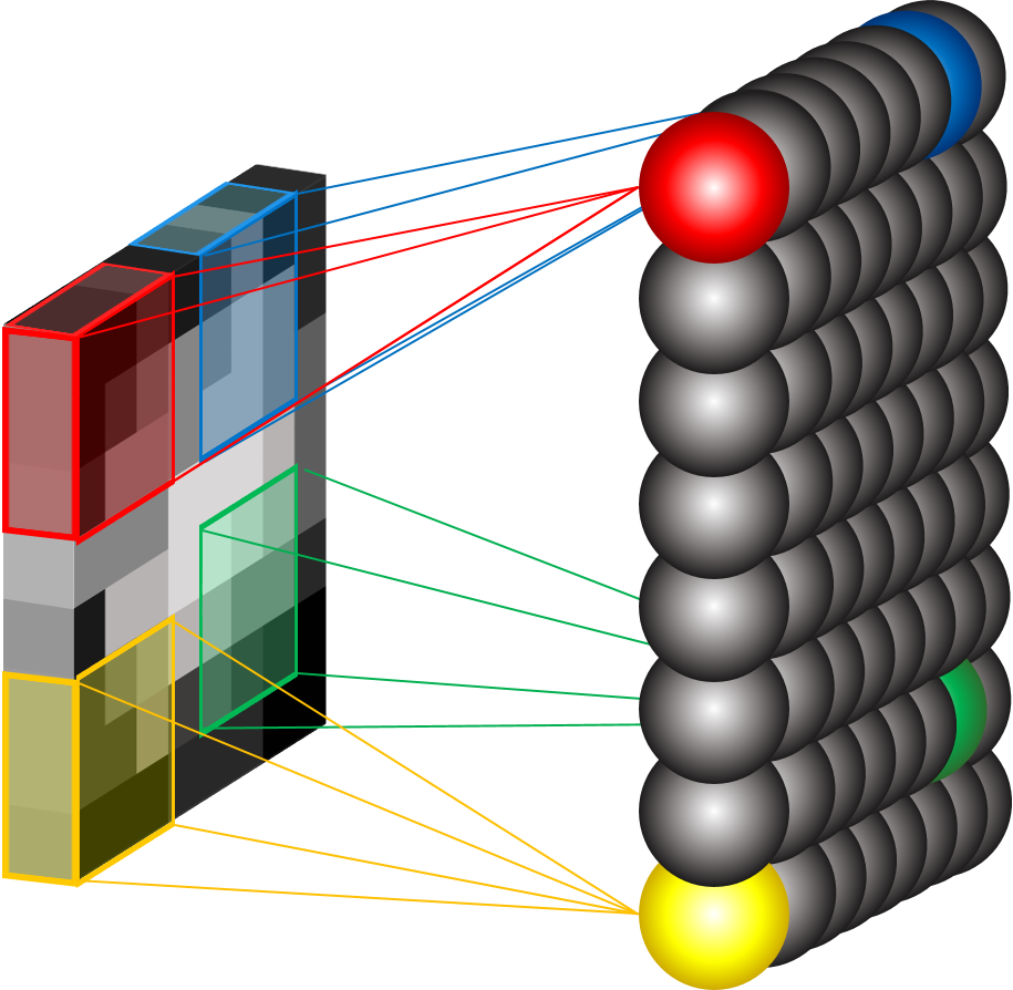
Hidden Layer Nodes in a CNN
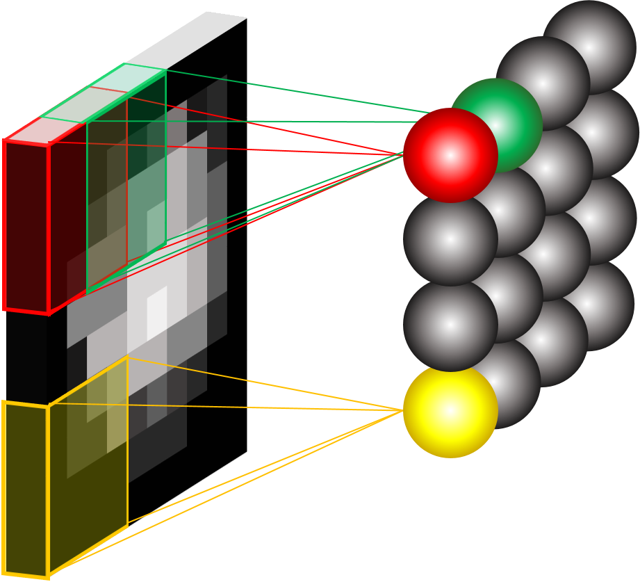
Increased stride means fewer hidden-layer nodes
These weights that connect to the nodes need to be learned in exactly the same way as in a regular neural network. The image is passed through these nodes (by being convolved with the weights a.k.a the kernel) and the result is compared to some output (the error of which is then backpropagated and optimised).
In reality, it isn’t just the weights or the kernel for one 2D set of nodes that has to be learned, there is a whole array of nodes which all look at the same area of the image (sometimes, but possibly incorrectly, called the receptive field*). Each of the nodes in this row (or fibre) tries to learn different kernels (different weights) that will show up some different features of the image, like edges. So the hidden-layer may look something more like this:
* Note: we’ll talk more about the receptive field after looking at the pooling layer below
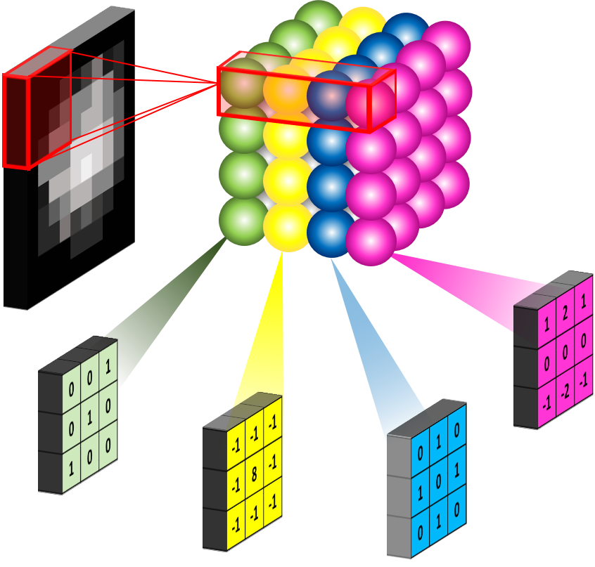
For a 2D image learning a set of kernels.
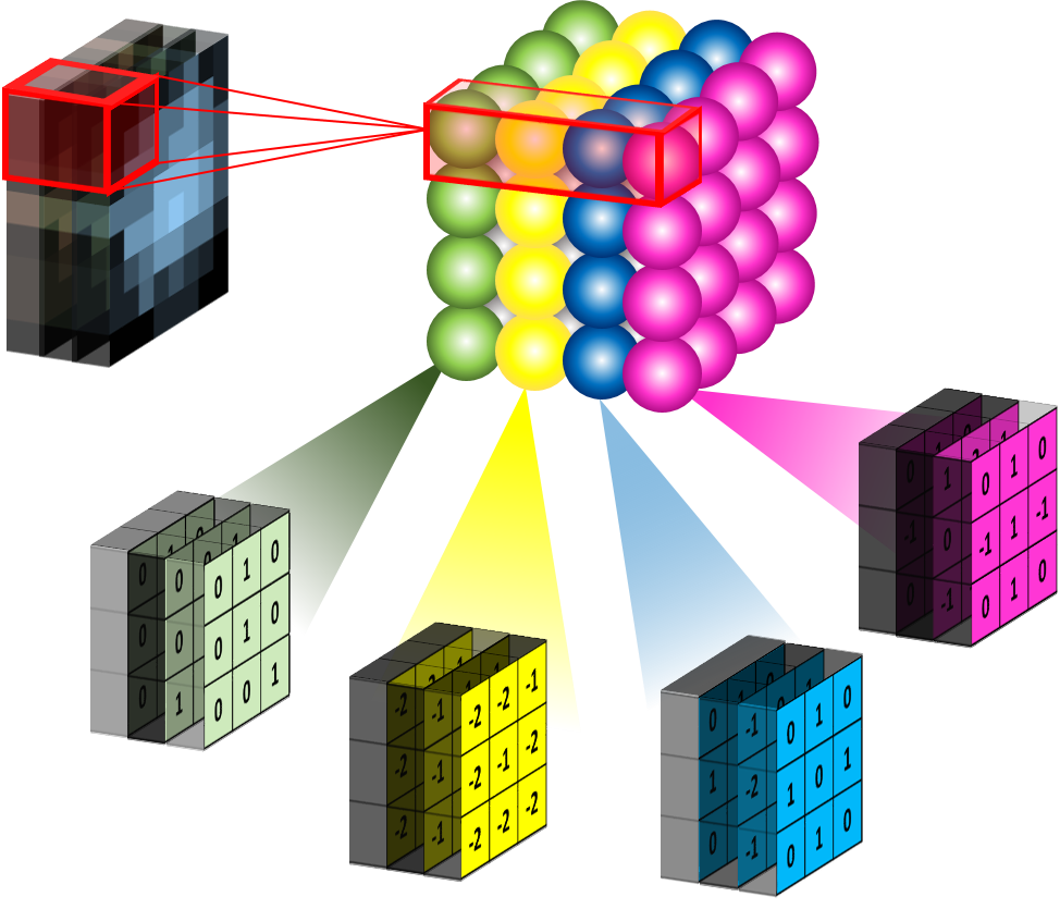
For a 3 channel RGB image the kernel becomes 3D.
Now this is why deep learning is called deep learning. Each hidden layer of the convolutional neural network is capable of learning a large number of kernels. The output from this hidden-layer is passed to more layers which are able to learn their own kernels based on the convolved image output from this layer (after some pooling operation to reduce the size of the convolved output). This is what gives the CNN the ability to see the edges of an image and build them up into larger features.
CNN Archiecture
It is the architecture of a CNN that gives it its power. A lot of papers that are puplished on CNNs tend to be about a new achitecture i.e. the number and ordering of different layers and how many kernels are learnt. Though often it’s the clever tricks applied to older architecures that really give the network power. Let’s take a look at the other layers in a CNN.
Layers
Input Layer
The input image is placed into this layer. It can be a single-layer 2D image (grayscale), 2D 3-channel image (RGB colour) or 3D. The main difference between how the inputs are arranged comes in the formation of the expected kernel shapes. Kernels need to be learned that are the same depth as the input i.e. 5 x 5 x 3 for a 2D RGB image with dimensions of 5 x 5.
Inputs to a CNN seem to work best when they’re of certain dimensions. This is because of the behviour of the convolution. Depending on the stride of the kernel and the subsequent pooling layers the outputs may become an “illegal” size including half-pixels. We’ll look at this in the pooling layer section.
Convolutional Layer
We’ve already looked at what the conv layer does. Just remember that it takes in an image e.g. [56 x 56 x 3] and assuming a stride of 1 and zero-padding, will produce an output of [56 x 56 x 32] if 32 kernels are being learnt. It’s important to note that the order of these dimensions can be important during the implementation of a CNN in Python. This is because there’s alot of matrix multiplication going on!
Non-linearity
The ‘non-linearity’ here isn’t its own distinct layer of the CNN, but comes as part of the convolution layer as it is done on the output of the neurons (just like a normal NN). By this, we mean “don’t take the data forwards as it is (linearity) let’s do something to it (non-linearlity) that will help us later on”.
In our neural network tutorials we looked at different activation functions. These each provide a different mapping of the input to an output, either to [-1 1], [0 1] or some other domain e.g the Rectified Linear Unit thresholds the data at 0: max(0,x). The ReLU is very popular as it doesn’t require any expensive computation and it’s been shown to speed up the convergence of stochastic gradient descent algorithms.
Pooling Layer
The pooling layer is key to making sure that the subsequent layers of the CNN are able to pick up larger-scale detail than just edges and curves. It does this by merging pixel regions in the convolved image together (shrinking the image) before attempting to learn kernels on it. Effectlively, this stage takes another kernel, say [2 x 2] and passes it over the entire image, just like in convolution. It is common to have the stride and kernel size equal i.e. a [2 x 2] kernel has a stride of 2. This example will half the size of the convolved image. The number of feature-maps produced by the learned kernels will remain the same as pooling is done on each one in turn. Thus the pooling layer returns an array with the same depth as the convolution layer. The figure below shows the principal.
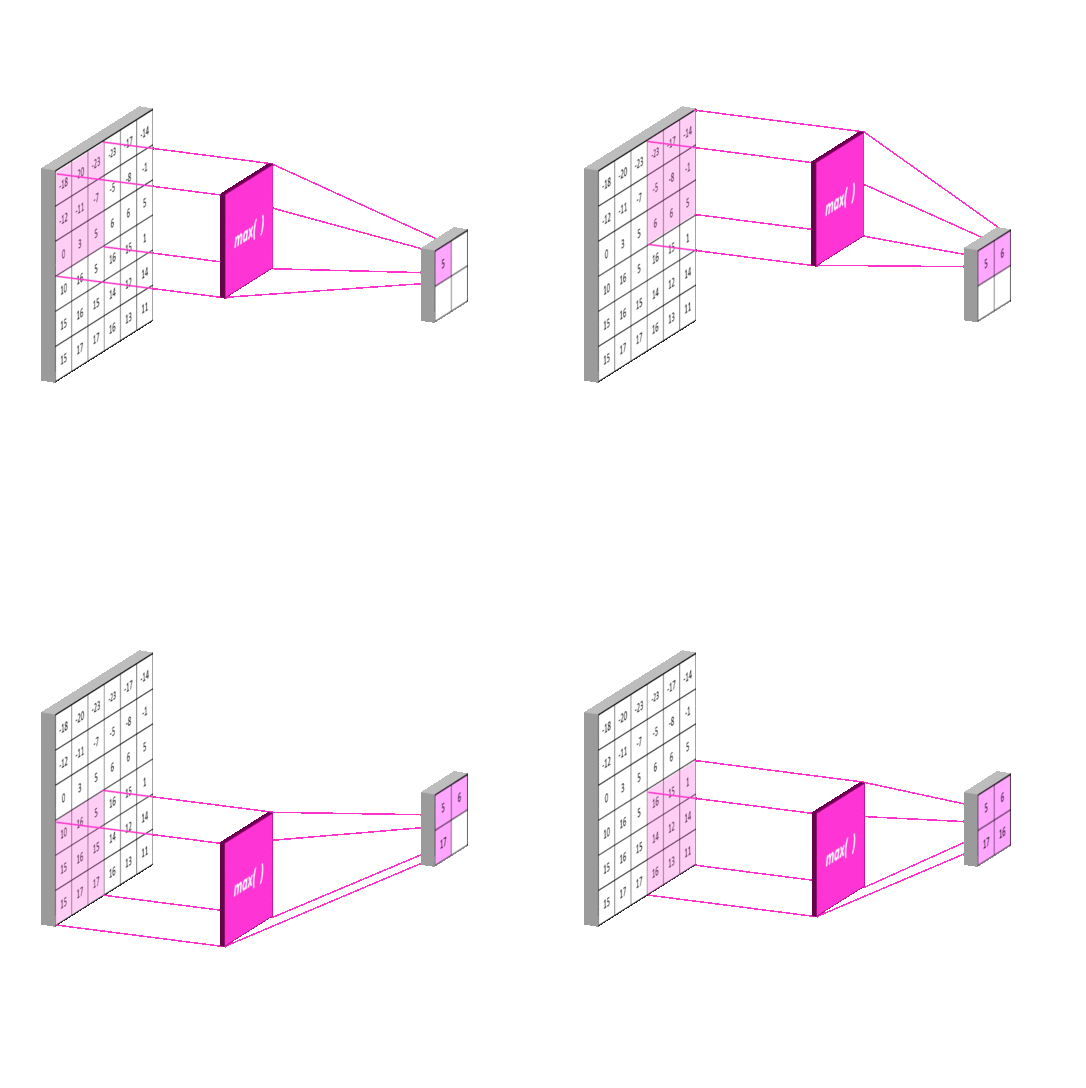
Max-pooling: Pooling using a "max" filter with stride equal to the kernel size
A Note on the Receptive Field
This is quite an important, but sometimes neglected, concept. We said that the receptive field of a single neuron can be taken to mean the area of the image which it can ‘see’. Each neuron therefore has a different receptive field. While this is true, the full impact of it can only be understood when we see what happens after pooling.
Let’s take an image of size [12 x 12] and a kernel size in the first conv layer of [3 x 3]. The output of the conv layer (assuming zero-padding and stride of 1) is going to be [12 x 12 x 10] if we’re learning 10 kernels. After pooling with a [3 x 3] kernel, we get an output of [4 x 4 x 10]. This gets fed into the next conv layer. Suppose the kernel in the second conv layer is [2 x 2], would we say that the receptive field here is also [2 x 2]? Well, some people do but, actually, no it’s not. In fact, a neuron in this layer is not just seeing the [2 x 2] area of the convolved image, it is actually seeing a [4 x 4] area of the original image too. That’s the [3 x 3] of the first layer for each of the pixels in the ‘receptive field’ of the second layer (remembering we had a stride of 1 in the first layer). Continuing this through the rest of the network, it is possible to end up with a final layer with a recpetive field equal to the size of the original image. Understanding this gives us the real insight to how the CNN works, building up the image as it goes.
Fully-connected (Dense) Layer
So this layer took me a while to figure out, despite its simplicity. If I take all of the say [3 x 3 x 64] featuremaps of my final pooling layer I have 3 x 3 x 64 = 576 different weights to consider and update. I need to make sure that my training labels match with the outputs from my output layer. We may only have 10 possibilities in our output layer (say the digits 0 - 9 in the classic MNIST number classification task). Thus we want the final numbers in our output layer to be [10,] and the layer before this to be [? x 10] where the ? represents the number of nodes in the layer before: the fully-connected (FC) layer. If there was only 1 node in this layer, it would have 576 weights attached to it - one for each of the weights coming from the previous pooling layer. This is not very useful as it won’t allow us to learn any combinations of these low-dimensional outputs. Increasing the number of neurons to say 1,000 will allow the FC layer to provide many different combinations of features and learn a more complex non-linear function that represents the feature space. The number of nodes in this layer can be whatever we want it to be and isn’t constrained by any previous dimensions - this is the thing that kept confusing me when I looked at other CNNs. Sometimes it’s also seen that there are two FC layers together, this just increases the possibility of learning a complex function. FC layers are 1D vectors.
However, FC layers act as ‘black boxes’ and are notoriously uninterpretable. They’re also prone to overfitting so dropout’ is often performed (discussed below).
Fully-connected as a Convolutional Layer
If the idea above doesn’t help you lets remove the FC layer and replace it with another convolutional layer. This is very simple - take the output from the pooling layer as before and apply a convolution to it with a kernel that is the same size as a featuremap in the pooling layer. For this to be of use, the input to the conv should be down to around [5 x 5] or [3 x 3] by making sure there have been enough pooling layers in the network. What does this achieve? By convolving a [3 x 3] image with a [3 x 3] kernel we get a 1 pixel output. There is no striding, just one convolution per featuremap. So our output from this layer will be a [1 x k] vector where k is the number of featuremaps. This is very similar to the FC layer, except that the output from the conv is only created from an individual featuremap rather than being connected to all of the featuremaps.
But, isn’t this more weights to learn? Yes, so it isn’t done. Instead, we perform either global average pooling or global max pooling where the global refers to a whole single feature map (not the whole set of feature maps). So we’re taking the average of all points in the feature and repeating this for each feature to get the [1 x k] vector as before. Note that the number of channels (kernels/features) in the last conv layer has to be equal to the number of outputs we want, or else we have to include an FC layer to change the [1 x k] vector to what we need.
This can be powerfull as we have represented a very large receptive field by a single pixel and also removed some spatial information that allows us to try and take into account translations of the input. We’re able to say, if the value of the output is high, that all of the featuremaps visible to this output have activated enough to represent a ‘cat’ or whatever it is we are training our network to learn.
Dropout Layer
The previously mentioned fully-connected layer is connected to all weights in the previous layer - this can be a very large number. As such, an FC layer is prone to overfitting meaning that the network won’t generalise well to new data. There are a number of techniques that can be used to reduce overfitting though the most commonly seen in CNNs is the dropout layer, proposed by Hinton. As the name suggests, this causes the network to ‘drop’ some nodes on each iteration with a particular probability. The keep probability is between 0 and 1, most commonly around 0.2-0.5 it seems. This is the probability that a particular node is dropped during training. When back propagation occurs, the weights connected to these nodes are not updated. They are readded for the next iteration before another set is chosen for dropout.
Output Layer
Of course depending on the purpose of your CNN, the output layer will be slightly different. In general, the output layer consists of a number of nodes which have a high value if they are ‘true’ or activated. Consider a classification problem where a CNN is given a set of images containing cats, dogs and elephants. If we’re asking the CNN to learn what a cat, dog and elephant looks like, output layer is going to be a set of three nodes, one for each ‘class’ or animal. We’d expect that when the CNN finds an image of a cat, the value at the node representing ‘cat’ is higher than the other two. This is the same idea as in a regular neural network. In fact, the FC layer and the output layer can be considered as a traditional NN where we also usually include a softmax activation function. Some output layers are probabilities and as such will sum to 1, whilst others will just achieve a value which could be a pixel intensity in the range 0-255. The output can also consist of a single node if we’re doing regression or deciding if an image belong to a specific class or not e.g. diseased or healthy. Commonly, however, even binary classificaion is proposed with 2 nodes in the output and trained with labels that are ‘one-hot’ encoded i.e. [1,0] for class 0 and [0,1] for class 1.
A Note on Back Propagation
I’ve found it helpful to consider CNNs in reverse. It didn’t sit properly in my mind that the CNN first learns all different types of edges, curves etc. and then builds them up into large features e.g. a face. It came up in a discussion with a colleague that we could consider the CNN working in reverse, and in fact this is effectively what happens - back propagation updates the weights from the final layer back towards the first. In fact, the error (or loss) minimisation occurs firstly at the final layer and as such, this is where the network is ‘seeing’ the bigger picture. The gradient (updates to the weights) vanishes towards the input layer and is greatest at the output layer. We can effectively think that the CNN is learning “face - has eyes, nose mouth” at the output layer, then “I don’t know what a face is, but here are some eyes, noses, mouths” in the previous one, then “What are eyes? I’m only seeing circles, some white bits and a black hole” followed by “woohoo! round things!” and initially by “I think that’s what a line looks like”. Possibly we could think of the CNN as being less sure about itself at the first layers and being more advanced at the end.
CNNs can be used for segmentation, classification, regression and a whole manner of other processes. On the whole, they only differ by four things:
- architecture (number and order of conv, pool and fc layers plus the size and number of the kernels)
- output (probabilitstic etc.)
- training method (cost or loss function, regularisation and optimiser)
- hyperparameters (learning rate, regularisation weights, batch size, iterations…)
There may well be other posts which consider these kinds of things in more detail, but for now I hope you have some insight into how CNNs function. Now, lets code it up…
comments powered by Disqus


