The 5th installment of our tutorial on implementing a neural network (NN) in Python. By the end of this tutorial, our NN should perform much more efficiently giving good results with fewer iterations. We will do this by implementing “momentum” into our network. We will also put in the other transfer functions for each layer.
Introduction
We’ve come so far! The intial maths was a bit of a slog, as was the vectorisation of that maths, but it was important to be able to implement our NN in Python which we did in our previous post. So what now? Well, you may have noticed when running the NN as it stands that it isn’t overly quick, depening on the randomly initialised weights, it may take the network the full number of maxIterations to converge, and then it may not converge at all! But there is something we can do about it. Let’s learn about, and implement, ‘momentum’.
Momentum
Background
Let’s revisit our equation for error in the NN:
This isn’t the only error function that could be used. In fact, there’s a whole field of study in NN about the best error or ‘optimisation’ function that should be used. This one tries to look at the sum of the squared-residuals between the outputs and the expected values at the end of each forward pass (the so-called $l_{2}$-norm). Others e.g. $l_{1}$-norm, look at minimising the sum of the absolute differences between the values themselves. There are more complex error (a.k.a. optimisation or cost) functions, for example those that look at the cross-entropy in the data. There may well be a post in the future about different cost-functions, but for now we will still focus on the equation above.
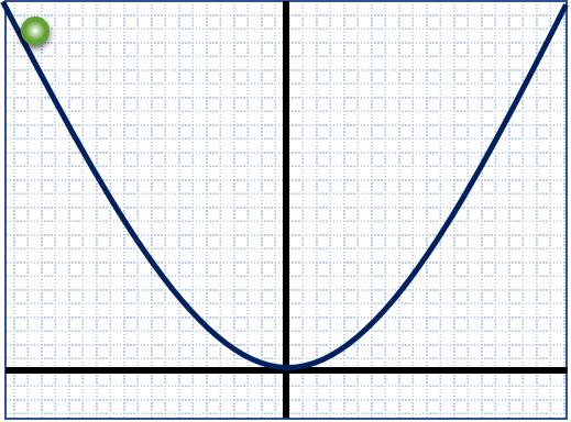
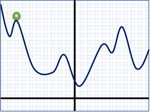
Now this function is described as a ‘convex’ function. This is an important property if we are to make our NN converge to the correct answer. Take a look at the two functions below:


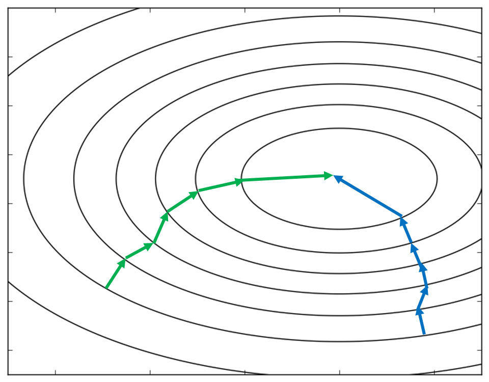
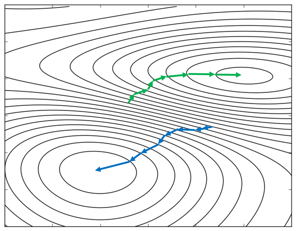
Let’s say that our current error was represented by the green ball. Our NN will calculate the gradient of its cost function at this point then look for the direction which is going to minimise the error i.e. go down a slope. The NN will feed the result into the back-propagation algorithm which will hopefully mean that on the next iteration, the error will have decreased. For a convex function, this is very straight forward, the NN just needs to keep going in the direction it found on the first run. But, look at the non-convex or stochastic function: our current error (green ball) sits at a point where either direction will take it to a lower error i.e. the gradient decreases on both sides. If the error goes to the left, it will hit one of the possible minima of the function, but this will be a higher minima (higher final error) than if the error had chosen the gradient to the right. Clearly the starting point for the error here has a big impact on the final result. Looking down at the 2D perspective (remembering that these are complex multi-dimensional functions), the non-convex case is clearly more ambiguous in terms of the location of the minimum and direction of descent. The convex function, however, nicely guides the error to the minimum with little care of the starting point.


So let’s focus on the convex case and explain what momentum is and why it works. I don’t think you’ll ever see a back propagation algorithm without momentum implemented in some way. In its simplest form, it modifies the weight-update equation:
by adding an extra momentum term:
The weight delta (the update amount to the weights after BP) now relies on its previous value i.e. the weight delta now at iteration $t$ requires the value of itself from $t-1$. The $m$ or momentum term, like the learning rate $\eta$ is just a small number between 0 and 1. What effect does this have?
Using prior information about the network is beneficial as it stops the network firing wildly into the unknown. If it can know the previous weights that have given the current error, it can keep the descent to the minimum roughly pointing in the same direction as it was before. The effect is that each iteration does not jump around so much as it would otherwise. In effect, the result is similar to that of the learning rate. We should be careful though, a large value for $m$ may cause the result to jump past the minimum and back again if combined with a large learning rate. We can think of momentum as changing the path taken to the optimum.
Momentum in Python
So, implementing momentum into our NN should be pretty easy. We will need to provide a momentum term to the backProp method of the NN and also create a new matrix in which to store the weight deltas from the current epoch for use in the subsequent one.
In the __init__ method of the NN, we need to initialise the previous weight matrix and then give them some values - they’ll start with zeros:
def __init__(self, numNodes):
	"""Initialise the NN - setup the layers and initial weights"""

	# Layer info
	self.numLayers = len(numNodes) - 1
	self.shape = numNodes

	# Input/Output data from last run
	self._layerInput = []
	self._layerOutput = []
	self._previousWeightDelta = []

	# Create the weight arrays
	for (l1,l2) in zip(numNodes[:-1],numNodes[1:]):
	    self.weights.append(np.random.normal(scale=0.1,size=(l2,l1+1)))
	    self._previousWeightDelta.append(np.zeros((l2,l1+1)))
The only other part of the NN that needs to change is the definition of backProp adding momentum to the inputs, and updating the weight equation. Finally, we make sure to save the current weights into the previous-weight matrix:
def backProp(self, input, target, trainingRate = 0.2, momentum=0.5):
	"""Get the error, deltas and back propagate to update the weights"""
	...
	weightDelta = trainingRate * thisWeightDelta + momentum * self._previousWeightDelta[index]

	self.weights[index] -= weightDelta

	self._previousWeightDelta[index] = weightDelta
Testing
Our default values for learning rate and momentum are 0.2 and 0,5 respectively. We can change either of these by including them in the call to backProp. Thi is the only change to the iteration process:
for i in range(maxIterations + 1):
    Error = NN.backProp(Input, Target, learningRate=0.2, momentum=0.5)
    if i % 2500 == 0:
        print("Iteration {0}\tError: {1:0.6f}".format(i,Error))
    if Error <= minError:
        print("Minimum error reached at iteration {0}".format(i))
        break

Iteration 100000	Error: 0.000076
Input 	Output 		Target
[0 0]	 [ 0.00491572] 	[ 0.]
[1 1]	 [ 0.00421318] 	[ 0.]
[0 1]	 [ 0.99586268] 	[ 1.]
[1 0]	 [ 0.99586257] 	[ 1.]
Feel free to play around with these numbers, however, it would be unlikely that much would change right now. I say this beacuse there is only so good that we can get when using only the sigmoid function as our activation function. If you go back and read the post on transfer functions you’ll see that it’s more common to use linear functions for the output layer. As it stands, the sigmoid function is unable to output a 1 or a 0 because it is asymptotic at these values. Therefore, no matter what learning rate or momentum we use, the network will never be able to get the best output.
This seems like a good time to implement the other transfer functions.
Transfer Functions
We’ve already gone through writing the transfer functions in Python in the transfer functions post. We’ll just put these under the sigmoid function we defined earlier. I’m going to use sigmoid, linear, gaussian and tanh here.
To modify the network, we need to assign each layer its own activation function, so let’s put that in the ‘layer information’ part of the __init__ method:
def __init__(self, layerSize, transferFunctions=None):
	"""Initialise the Network"""

	# Layer information
	self.numLayers = len(numLayers) - 1
	self.shape = numNodes

	if transferFunctions is None:
	    layerTFs = []
	    for i in range(self.numLayers):
		if i == self.numLayers - 1:
		    layerTFs.append(linear)
		else:
		    layerTFs.append(sigmoid)
	else:
            if len(numNodes) != len(transferFunctions):
                raise ValueError("Number of transfer functions must match the number of layers: minus input layer")
            elif transferFunctions[0] is not None:
                raise ValueError("The Input layer doesn't need a a transfer function: give it [None,...]")
            else:
                layerTFs = transferFunctions[1:]

	self.tFunctions = layerTFs
Let’s go through this. We input into the initialisation a parameter called transferFunctions with a default value of None. If the default it taken, or if the parameter is ommitted, we set some defaults. for each layer, we use the sigmoid function, unless its the output layer where we will use the linear function. If a list of transferFunctions is given, first, check that it’s a ‘legal’ input. If the number of functions in the list is not the same as the number of layers (given by numNodes) then throw an error. Also, if the first function in the list is not "None" throw an error, because the first layer shouldn’t have an activation function (it is the input layer). If those two things are fine, go ahead and store the list of functions as layerTFs without the first (element 0) one.
We next need to replace all of our calls directly to sigmoid and its derivative. These should now refer to the list of functions via an index that depends on the number of the current layer. There are 3 instances of this in our NN: 1 in the forward pass where we call sigmoid directly, and 2 in the backProp method where we call the derivative at the output and hidden layers. so sigmoid(layerInput) for example should become:
self.tFunctions[index](layerInput)
Check the updated code here if that’s confusing.
Let’s test this out! We’ll modify the call to initialising the NN by adding a list of functions like so:
Input = np.array([[0,0],[1,1],[0,1],[1,0]])
Target = np.array([[0.0],[0.0],[1.0],[1.0]])
transferFunctions = [None, sigmoid, linear]

NN = backPropNN((2,2,1), transferFunctions)
Running the NN like this with the default learning rate and momentum should provide you with an immediate performance boost simply becuase with the linear function we’re now able to get closer to the target values, reducing the error.
Iteration 0	Error: 1.550211
Iteration 2500	Error: 1.000000
Iteration 5000	Error: 0.999999
Iteration 7500	Error: 0.999999
Iteration 10000	Error: 0.999995
Iteration 12500	Error: 0.999969
Minimum error reached at iteration 14543
Input 	Output 		Target
[0 0]	 [ 0.0021009] 	[ 0.]
[1 1]	 [ 0.00081154] 	[ 0.]
[0 1]	 [ 0.9985881] 	[ 1.]
[1 0]	 [ 0.99877479] 	[ 1.]
Play around with the number of layers and different combinations of transfer functions as well as tweaking the learning rate and momentum. You’ll soon get a feel for how each changes the performance of the NN.
comments powered by Disqus


