This is the first part of a series of tutorials on Simple Neural Networks (NN). Tutorials on neural networks (NN) can be found all over the internet. Though many of them are the same, each is written (or recorded) slightly differently. This means that I always feel like I learn something new or get a better understanding of things with every tutorial I see. I’d like to make this tutorial as clear as I can, so sometimes the maths may be simplistic, but hopefully it’ll give you a good unserstanding of what’s going on. Please let me know if any of the notation is incorrect or there are any mistakes - either comment or use the contact page on the left.
- Neural Network Architecture
- Transfer Function
- Feed-forward
- Error
- Back Propagation - the Gradients
- Bias
- Back Propagaton - the Algorithm
1. Neural Network Architecture
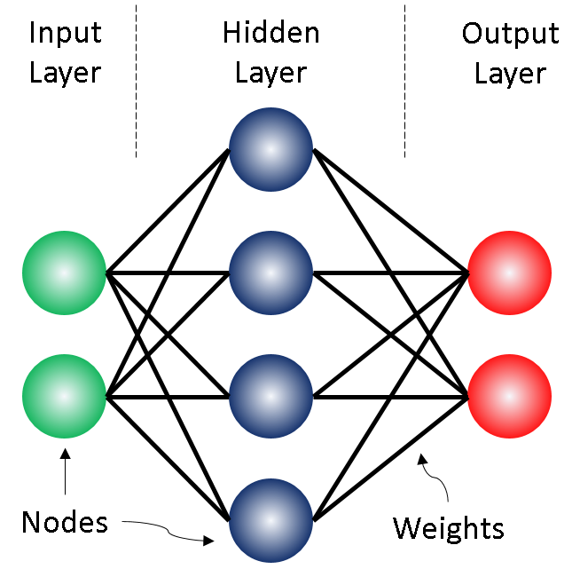
By now, you may well have come across diagrams which look very similar to the one below. It shows some input node, connected to some output node via an intermediate node in what is called a ‘hidden layer’ - ‘hidden’ because in the use of NN only the input and output is of concern to the user, the ‘under-the-hood’ stuff may not be interesting to them. In real, high-performing NN there are usually more hidden layers.

When we train our network, the nodes in the hidden layer each perform a calculation using the values from the input nodes. The output of this is passed on to the nodes of the next layer. When the output hits the final layer, the ‘output layer’, the results are compared to the real, known outputs and some tweaking of the network is done to make the output more similar to the real results. This is done with an algorithm called back propagation. Before we get there, lets take a closer look at these calculations being done by the nodes.
2. Transfer Function
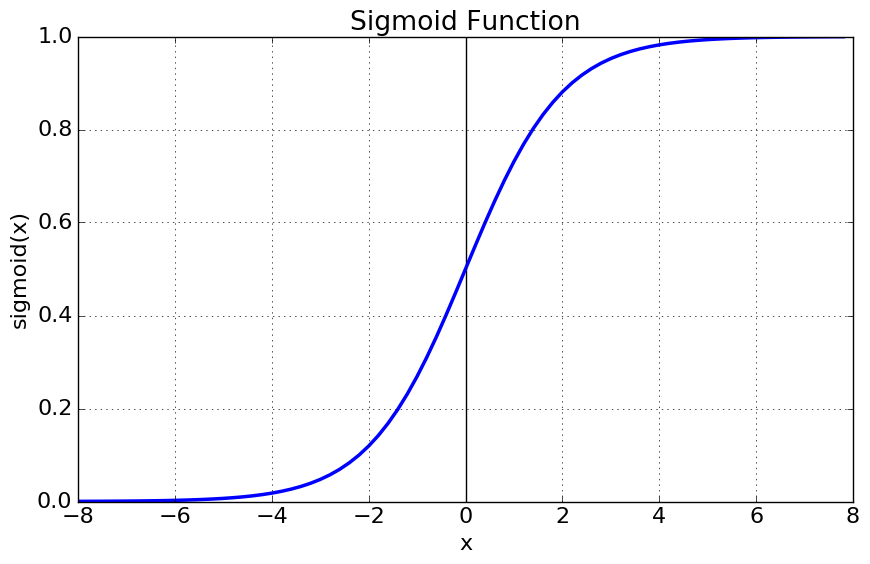
At each node in the hidden and output layers of the NN, an activation or transfer function is executed. This function takes in the output of the previous node, and multiplies it by some weight. These weights are the lines which connect the nodes. The weights that come out of one node can all be different, that is they will activate different neurons. There can be many forms of the transfer function, we will first look at the sigmoid transfer function as it seems traditional.

As you can see from the figure, the sigmoid function takes any real-valued input and maps it to a real number in the range $(0 \ 1)$ - i.e. between, but not equal to, 0 and 1. We can think of this almost like saying ‘if the value we have maps to an output near 1, this node fires, if it maps to an output near 0, the node does not fire’. The equation for this sigmoid function is:
We need to have the derivative of this transfer function so that we can perform back propagation later on. This is the process where by the connections in the network are updated to tune the performance of the NN. We’ll talk about this in more detail later, but let’s find the derivative now.
Therefore, we can write the derivative of the sigmoid function as:
The sigmoid function has the nice property that its derivative is very simple: a bonus when we want to hard-code this into our NN later on. Now that we have our activation or transfer function selected, what do we do with it?
3. Feed-forward
During a feed-forward pass, the network takes in the input values and gives us some output values. To see how this is done, let’s first consider a 2-layer neural network like the one in Figure 1. Here we are going to refer to:
- $i$ - the $i^{\text{th}}$ node of the input layer $I$
- $j$ - the $j^{\text{th}}$ node of the hidden layer $J$
- $k$ - the $k^{\text{th}}$ node of the input layer $K$
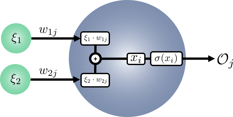
The activation function at a node $j$ in the hidden layer takes the value:
where $\xi_{i}$ is the value of the $i^{\text{th}}$ input node and $w_{i j}$ is the weight of the connection between $i^{\text{th}}$ input node and the $j^{\text{th}}$ hidden node. In short: at each hidden layer node, multiply each input value by the connection received by that node and add them together.
Note: the weights are initisliased when the network is setup. Sometimes they are all set to 1, or often they’re set to some small random value.
We apply the activation function on $x_{j}$ at the $j^{\text{th}}$ hidden node and get:
$\mathcal{O}_{j}$ is the output of the $j^{\text{th}}$ hidden node. This is calculated for each of the $j$ nodes in the hidden layer. The resulting outputs now become the input for the next layer in the network. In our case, this is the final output later. So for each of the $k$ nodes in $K$:
As we’ve reached the end of the network, this is also the end of the feed-foward pass. So how well did our network do at getting the correct result $\mathcal{O}_{k}$? As this is the training phase of our network, the true results will be known an we cal calculate the error.
4. Error
We measure error at the end of each foward pass. This allows us to quantify how well our network has performed in getting the correct output. Let’s define $t_{k}$ as the expected or target value of the $k^{\text{th}}$ node of the output layer $K$. Then the error $E$ on the entire output is:
Dont’ be put off by the random 1⁄2 in front there, it’s been manufactured that way to make the upcoming maths easier. The rest of this should be easy enough: get the residual (difference between the target and output values), square this to get rid of any negatives and sum this over all of the nodes in the output layer.
Good! Now how does this help us? Our aim here is to find a way to tune our network such that when we do a forward pass of the input data, the output is exactly what we know it should be. But we can’t change the input data, so there are only two other things we can change:
- the weights going into the activation function
- the activation function itself
We will indeed consider the second case in another post, but the magic of NN is all about the weights. Getting each weight i.e. each connection between nodes, to be just the perfect value, is what back propagation is all about. The back propagation algorithm we will look at in the next section, but lets go ahead and set it up by considering the following: how much of this error $E$ has come from each of the weights in the network?
We’re asking, what is the proportion of the error coming from each of the $W_{jk}$ connections between the nodes in layer $J$ and the output layer $K$. Or in mathematical terms:
If you’re not concerned with working out the derivative, skip this highlighted section.
- the weight $w_{1k}$ does not affect connection $w_{2k}$ therefore the change in $W_{jk}$ with respect to any node other than the current $k$ is zero. Thus the summation goes away:
- apply the power rule knowing that $t_{k}$ is a constant:
- the leftover derivative is the chage in the output values with respect to the weights. Substituting $ \mathcal{O}_{k} = \sigma(x_{k}) $ and the sigmoid derivative $\sigma^{\prime}( x ) = \sigma (x ) \left( 1 - \sigma ( x ) \right)$:
- the final derivative, the input value $x_{k}$ is just $\mathcal{O}_{j} W_{jk}$ i.e. output of the previous layer times the weight to this layer. So the change in $\mathcal{O}_{j} w_{jk}$ with respect to $w_{jk}$ just gives us the output value of the previous layer $ \mathcal{O}_{j} $ and so the full derivative becomes:
We can replace the sigmoid function with the output of the layer
The derivative of the error function with respect to the weights is then:
We group the terms involving $k$ and define:
And therefore:
So we have an expression for the amount of error, called ‘deta’ ($\delta_{k}$), on the weights from the nodes in $J$ to each node $k$ in $K$. But how does this help us to improve out network? We need to back propagate the error.
5. Back Propagation - the gradients
Back propagation takes the error function we found in the previous section, uses it to calculate the error on the current layer and updates the weights to that layer by some amount.
So far we’ve only looked at the error on the output layer, what about the hidden layer? This also has an error, but the error here depends on the output layer’s error too (because this is where the difference between the target $t_{k}$ and output $\mathcal{O}_{k}$ can be calculated). Lets have a look at the error on the weights of the hidden layer $W_{ij}$:
Now, unlike before, we cannot just drop the summation as the derivative is not directly acting on a subscript $k$ in the summation. We should be careful to note that the output from every node in $J$ is actually connected to each of the nodes in $K$ so the summation should stay. But we can still use the same tricks as before: lets use the power rule again and move the derivative inside (because the summation is finite):
Again, we substitute $\mathcal{O}_{k} = \sigma( x_{k})$ and its derivative and revert back to our output notation:
This still looks familar from the output layer derivative, but now we’re struggling with the derivative of the input to $k$ i.e. $x_{k}$ with respect to the weights from $I$ to $J$. Let’s use the chain rule to break apart this derivative in terms of the output from $J$:
The change of the input to the $k^{\text{th}}$ node with respect to the output from the $j^{\text{th}}$ node is down to a product with the weights, therefore this derivative just becomes the weights $W_{jk}$. The final derivative has nothing to do with the subscript $k$ anymore, so we’re free to move this around - lets put it at the beginning:
Lets finish the derivatives, remembering that the output of the node $j$ is just $\mathcal{O}_{j} = \sigma(x_{j}) $ and we know the derivative of this function too:
The final derivative is straightforward too, the derivative of the input to $j$ with repect to the weights is just the previous input, which in our case is $\mathcal{O}_{i}$,
Almost there! Recall that we defined $\delta_{k}$ earlier, lets sub that in:
To clean this up, we now define the ‘delta’ for our hidden layer:
Thus, the amount of error on each of the weights going into our hidden layer:
Note: the reason for the name back propagation is that we must calculate the errors at the far end of the network and work backwards to be able to calculate the weights at the front.
6. Bias
Lets remind ourselves what happens inside our hidden layer nodes:

- Each feature $\xi_{i}$ from the input layer $I$ is multiplied by some weight $w_{ij}$
- These are added together to get $x_{i}$ the total, weighted input from the nodes in $I$
- $x_{i}$ is passed through the activation, or transfer, function $\sigma(x_{i})$
- This gives the output $\mathcal{O}_{j}$ for each of the $j$ nodes in hidden layer $J$
- $\mathcal{O}_{j}$ from each of the $J$ nodes becomes $\xi_{j}$ for the next layer
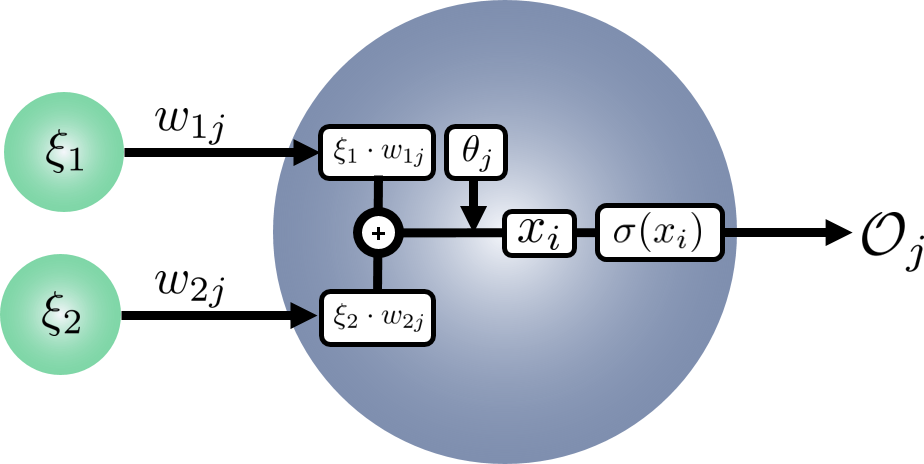
When we talk about the bias term in NN, we are talking about an additional parameter that is inluded in the summation of step 2 above. The bias term is usually denoted with the symbol $\theta$ (theta). It’s function is to act as a threshold for the activation (transfer) function. It is given the value of 1 and is not connected to anything else. As such, this means that any derivative of the node’s output with respect to the bias term would just give a constant, 1. This allows us to just think of the bias term as an output from the node with the value of 1. This will be updated later during backpropagation to change the threshold at which the node fires.
Lets update the equation for $x_{i}$:
and put it on the diagram:

7. Back Propagation - the algorithm
Now we have all of the pieces! We’ve got the initial outputs after our feed-forward, we have the equations for the delta terms (the amount by which the error is based on the different weights) and we know we need to update our bias term too. So what does it look like:
- Input the data into the network and feed-forward
For each of the output nodes calculate:
$$ \delta_{k} = \mathcal{O}_{k} \left( 1 - \mathcal{O}_{k} \right) \left( \mathcal{O}_{k} - t_{k} \right) $$For each of the hidden layer nodes calculate:
$$ \delta_{j} = \mathcal{O}_{i} \left( 1 - \mathcal{O}_{j} \right) \sum_{k \in K} \delta_{k} W_{jk} $$Calculate the changes that need to be made to the weights and bias terms:
$$ \begin{align} \Delta W &= -\eta \ \delta_{l} \ \mathcal{O}_{l-1} \\ \Delta\theta &= -\eta \ \delta_{l} \end{align} $$Update the weights and biases across the network:
$$ \begin{align} W + \Delta W &\rightarrow W \\ \theta + \Delta\theta &\rightarrow \theta \end{align} $$
Here, $\eta$ is just a small number that limit the size of the deltas that we compute: we don’t want the network jumping around everywhere. The $l$ subscript denotes the deltas and output for that layer $l$. That is, we compute the delta for each of the nodes in a layer and vectorise them. Thus we can compute the element-wise product with the output values of the previous layer and get our update $\Delta W$ for the weights of the current later. Similarly with the bias term.
This algorithm is looped over and over until the error between the output and the target values is below some set threshold. Depending on the size of the network i.e. the number of layers and number of nodes per layer, it can take a long time to complete one ‘epoch’ or run through of this algorithm.
Some of the ideas and notation in this tutorial comes from the good videos by Ryan Harris
comments powered by Disqus


