This is the final part in our series on Generative Adversarial Networks (GAN). We will write our training script and look at how to run the GAN. We will also take a look at the results we get out. Can you tell the difference between the real and generated faces?
Introduction
In this series we started out with a background to GAN including some of the mathematics behind them. We then downloaded and processed our dataset. In the subsequent posts, we wrote some image helper functions before completing some data processing functions and the GAN Class itself.
In this final post, we will create the training script and visualise some of the results we get out.
Training Script
The training script is here: `gantut_trainer.py’.
It’s only short, so there isn’t anything to fill in, but let’s take a look. We need to make sure we import the GAN class from our completed gantut_gan.py file.
Note: If you’re using the files called gantut_*_complete.py you’ll need to modify this line (add the _complete). Otherwise, just make sure it’s looking for the correctly named file where your GAN class is written.
#!/usr/bin/python

import os
import numpy as  np
import tensorflow as tf

from gantut_gan import DCGAN
The ‘shebang’ on the first line allows us to call this script from the terminal without typing python first. This is a useful line if you’re going to run this network on a cluster of computers where you will probably need to create your own python (or conda) virtual environment first. This line will be changed to point to the specific python installation that you want to use to run the script
Note: I’ll add this note here. The network will take a long time to train. If you have access to a cluster, I recommend using it.
Next, we define the possible ‘flags’ or attributes that we need the network to take:
#DEFINE THE FLAGS FOR RUNNING SCRIPT FROM THE TERMINAL
# ARG1 = NAME OF THE FLAG
# ARG2 = DEFAULT VALUE
# ARG3 = DESCRIPTION
flags = tf.app.flags
flags.DEFINE_integer("epoch", 20, "Number of epochs to train [20]")
flags.DEFINE_float("learning_rate", 0.0002, "Learning rate for adam optimiser [0.0002]")
flags.DEFINE_float("beta1", 0.5, "Momentum term for adam optimiser [0.5]")
flags.DEFINE_integer("train_size", np.inf, "The size of training images [np.inf]")
flags.DEFINE_integer("batch_size", 64, "The batch-size (number of images to train at once) [64]")
flags.DEFINE_integer("image_size", 64, "The size of the images [n x n] [64]")
flags.DEFINE_string("dataset", "lfw-aligned-64", "Dataset directory.")
flags.DEFINE_string("checkpoint_dir", "checkpoint", "Directory name to save the checkpoints [checkpoint]")
flags.DEFINE_string("sample_dir", "samples", "Directory name to save the image samples [samples]")
FLAGS = flags.FLAGS
Here, we’re using the tf.flags module (which is a wrapper for argparse) that takes arguments that trail the script name in the terminal and turn them into variables we can use in the network. The format for each argument is:
flags.DEFINE_datatype(name, default_value, description)
Where datatype is what is expected (an integer, float, string etc.), name is what the resulting variable will be called, default_value is… the default value in case it’s not explicitly defined at runtime, and description is a useful descriptor of what this argument does. We package all these variables into one (called FLAGS) that can be called later to assign values.
Notice that the name here is the same as those we wrote in the __init__ method of our GAN class because these will be used to initialise the GAN.
Our network will need folders to output to and also to check whether there’s an existing checkpoint that can be loaded (rather than doing it all over again).
#CREATE SOME FOLDERS FOR THE DATA
if not os.path.exists(FLAGS.checkpoint_dir):
    os.makedirs(FLAGS.checkpoint_dir)
if not os.path.exists(FLAGS.sample_dir):
    os.makedirs(FLAGS.sample_dir)
Even though we’ve just defined some variables for our network, there are plenty of others in the Graph that need some default value. TensorFlow has a handy function for that:
# GET ALL OF THE OPTIONS FOR TENSORFLOW RUNTIME
config = tf.ConfigProto(intra_op_parallelism_threads=8)
Tip: I’ve included the intra_op_parallelism_threads argument to tf.ConfigProto because TensorFlow has the power to take over as many cores as it can see when it’s running. This may not be a problem if you’re not using your machine too much, but if you’re running on a cluster, TF will ignore the ‘requested’ number of cpus/gpus and leech into other cores. Setting intra_op_parallelism_threads to the correct number of threads stops this from happening.
Finally, we initialise the TensorFlow session (with out config above), initialise the GAN and pass the flags to the .train method of the GAN class.
Tip: It is good to initialise the session in this way with with because it will be automatically closed when the GAN training is finished.
with tf.Session(config=config) as sess:
    #INITIALISE THE GAN BY CREATING A NEW INSTANCE OF THE DCGAN CLASS
    dcgan = DCGAN(sess, image_size=FLAGS.image_size, batch_size=FLAGS.batch_size,
                  is_crop=False, checkpoint_dir=FLAGS.checkpoint_dir)

    #TRAIN THE GAN
    dcgan.train(FLAGS)
Training
This is it! 5 posts later and we can train our GAN. From our terminal, we are going to call the training script gantut_trainer.py and pass it a couple of arguments:
~/GAN/gantut_trainer.py --dataset ~/GAN/aligned --epoch 20
Of course, if you’ve put your aligned training set somewhere else, make sure that path goes into the --dataset flag. The other flags can be set to default because that’s how we’ve written our GAN class. Now 20 epochs will take a seriously long time (it look me nearly 4 days using 12 cores on a cluster).
There will be 3 folders of output from the GAN:
logs- where the logs from the training will be saved. These can be viewed with TensorBoardcheckpoints- where the model itself is savedsamples- this is where the image array we created ingantut_imgfuncs.pywill be output to every so often.
Logs
Whilst the network is training (if you’re doing it locally) you can pull up tensorboard and watch how the training is progressing. From the terminal:
tensorboard --logdir="~/GAN/logs"
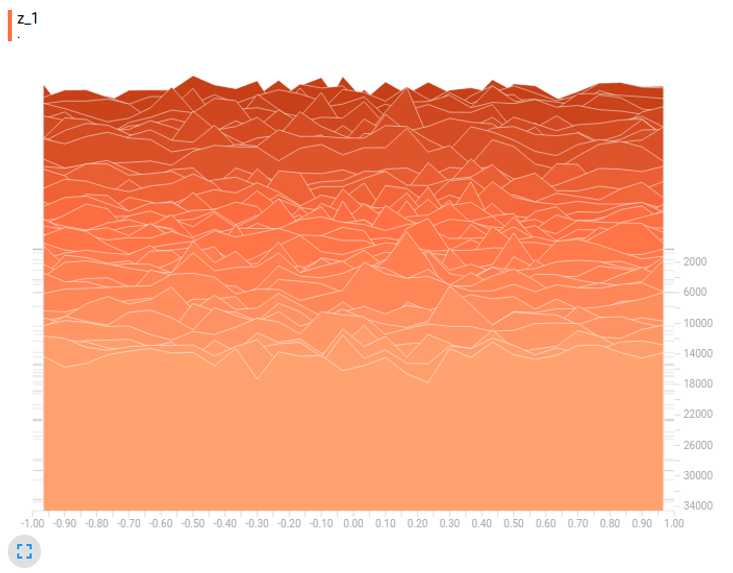
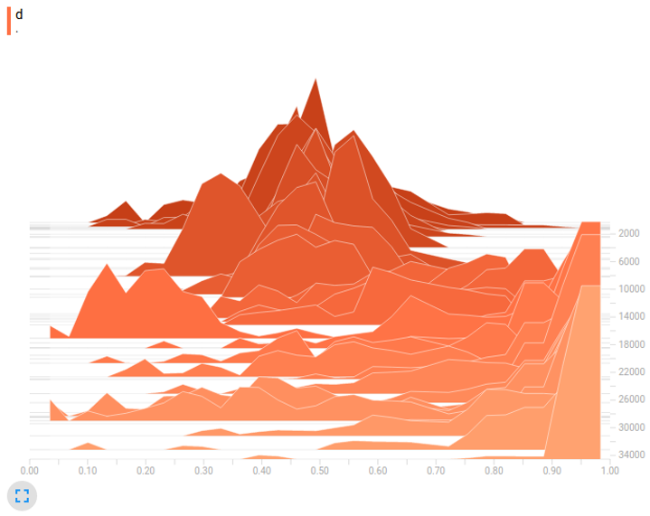
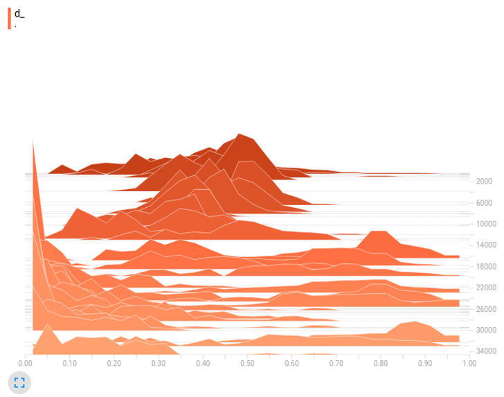
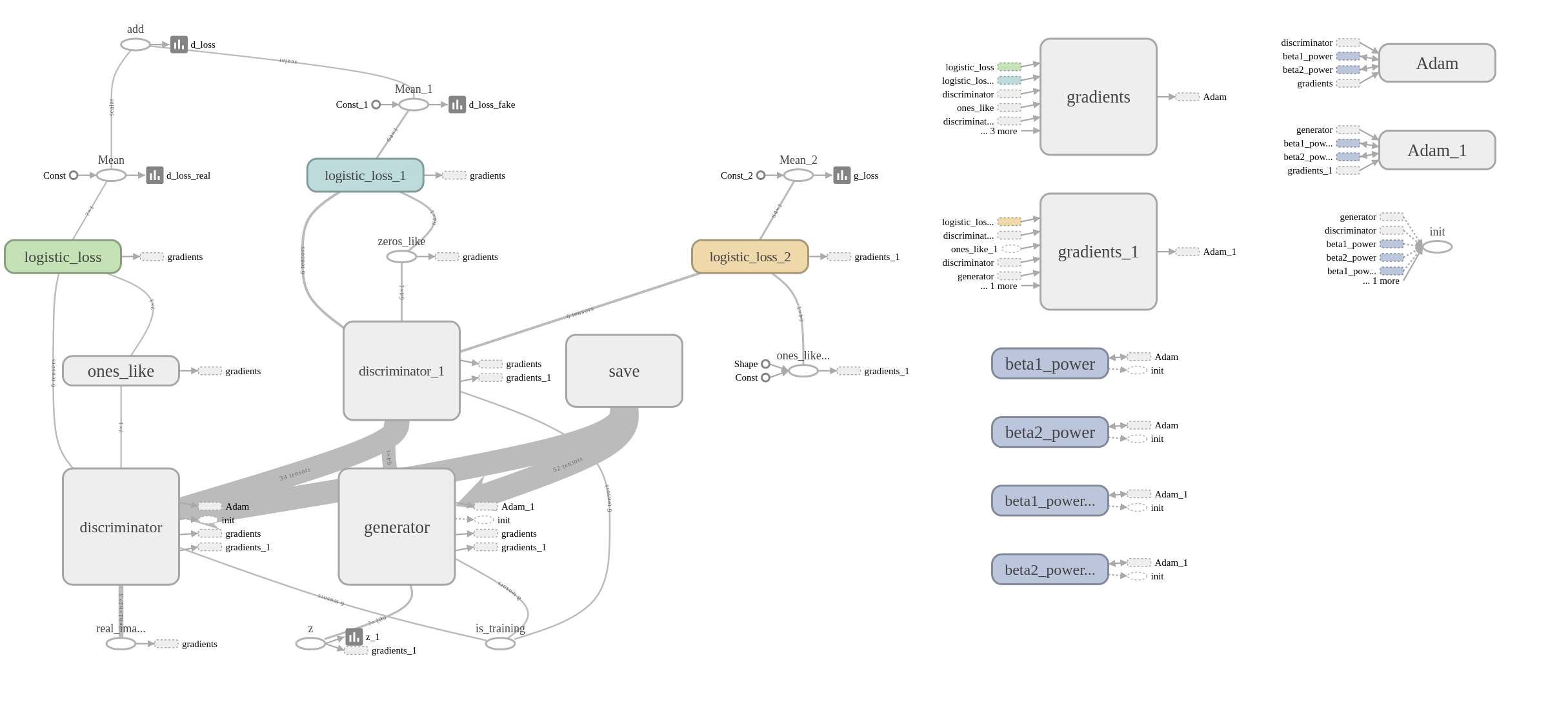
Follow the link it spits out and you’ll be presented with a lot of information about the network. You will find graphs of the loss-functions under ‘scalars’, some examples from the generator under ‘images’ and the Graph itself is nicely represented under ‘graph’. ‘Histograms’ show how the distributions are changing over time. We can see in these that our noise distribution $p_{z}$ is uniform (which is what we defined) and that the real and fake images take values around 1 and 0 at the discriminator, as we also described in part 1.
Results
Here it is, the output from our GAN (after 14 epochs in this case) showing how well the network has learned how to create faces. It may take longer than expect to load as I’ve tried to preserve quality.
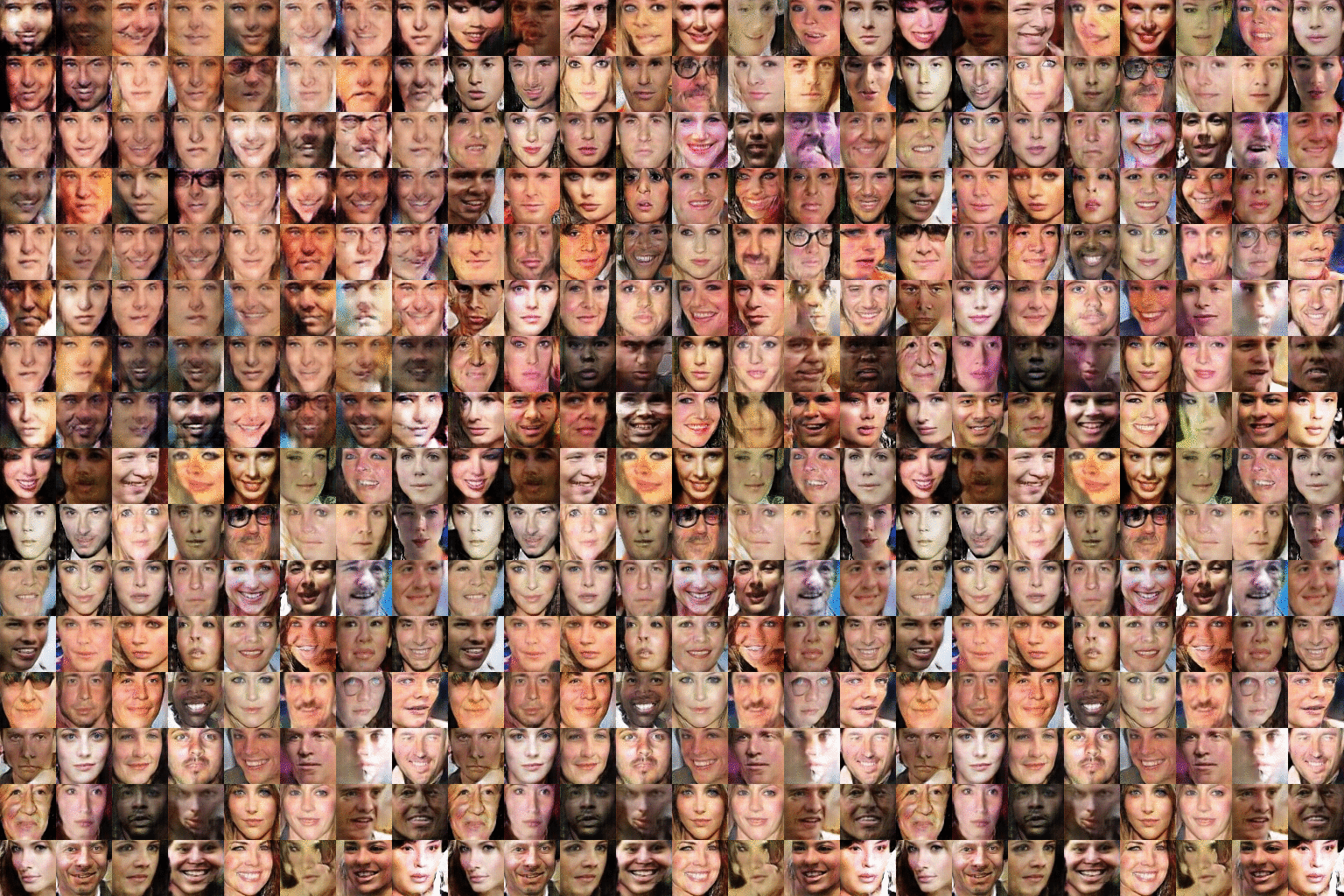
We can see that some of the faces are still not quite there yet, but there are a few that are unbelieveably realistic. In fact, we can perform a kind of ‘Turing Test’ on this data. The Turing Test, put simply, is that if a user is unable to reliably tell the difference between a computer and human performing the same task, then the computer has passed the Turing Test.
Have a go at the test below: study each face, decide if it is a real or fake image; then click on the image to reveal the true result. If you only guess 50% or less, then the computer has passed this simplistic Turing Test.
(opens in a new window)
Conclusion
So it looks great, but what was the point? Well, remember back to part 1 - GANs and other generative networks are used for image completion. We can use the fact that our network has learned what a face should look like to ‘fill-in’ any missing bits. Lets say someone has a large tattoo across their face, we can reconstruct what the skin would look like without it. Or maybe we have an amazing photo, with a beautiufl background, but we’re not smiling: the GAN can reconstruct a smile. More advanced work can include learning what glasses are and putting them onto other faces.
Again, for credit, this series is based on the main code by carpedm20 and inspired from the blog of B. Amos.
GANs are powerful networks, but work in a relatively simple way by trying to trick a discriminator by generating more and more realistic-looking images.
comments powered by Disqus


