A Simple Neural Network - Vectorisation

Simplifying the NN maths ready for coding

The third in our series of tutorials on Simple Neural Networks. This time, we’re looking a bit deeper into the maths, specifically focusing on vectorisation. This is an important step before we can translate our maths in a functioning script in Python.

So we’ve been through the maths of a neural network (NN) using back propagation and taken a look at the different activation functions that we could implement. This post will translate the mathematics into Python which we can piece together at the end into a functioning NN!

Forward Propagation

Let’s remimnd ourselves of our notation from our 2 layer network in the maths tutorial:

  • I is our input layer
  • J is our hidden layer
  • $w_{ij}$ is the weight connecting the $i^{\text{th}}$ node in in $I$ to the $j^{\text{th}}$ node in $J$
  • $x_{j}$ is the total input to the $j^{\text{th}}$ node in $J$

So, assuming that we have three features (nodes) in the input layer, the input to the first node in the hidden layer is given by:

$$ x_{1} = \mathcal{O}_{1}^{I} w_{11} + \mathcal{O}_{2}^{I} w_{21} + \mathcal{O}_{3}^{I} w_{31} $$

Lets generalise this for any connected nodes in any layer: the input to node $j$ in layer $l$ is:

$$ x_{j} = \mathcal{O}_{1}^{l-1} w_{1j} + \mathcal{O}_{2}^{l-1} w_{2j} + \mathcal{O}_{3}^{l-1} w_{3j} $$

But we need to be careful and remember to put in our bias term $\theta$. In our maths tutorial, we said that the bias term was always equal to 1; now we can try to understand why.

We could just add the bias term onto the end of the previous equation to get:

$$ x_{j} = \mathcal{O}_{1}^{l-1} w_{1j} + \mathcal{O}_{2}^{l-1} w_{2j} + \mathcal{O}_{3}^{l-1} w_{3j} + \theta_{i} $$

If we think more carefully about this, what we are really saying is that “an extra node in the previous layer, which always outputs the value 1, is connected to the node $j$ in the current layer by some weight $w_{4j}$“. i.e. $1 \cdot w_{4j}$:

$$ x_{j} = \mathcal{O}_{1}^{l-1} w_{1j} + \mathcal{O}_{2}^{l-1} w_{2j} + \mathcal{O}_{3}^{l-1} w_{3j} + 1 \cdot w_{4j} $$

By the magic of matrix multiplication, we should be able to convince ourselves that:

$$ x_{j} = \begin{pmatrix} w_{1j} &w_{2j} &w_{3j} &w_{4j} \end{pmatrix} \begin{pmatrix} \mathcal{O}_{1}^{l-1} \\ \mathcal{O}_{2}^{l-1} \\ \mathcal{O}_{3}^{l-1} \\ 1 \end{pmatrix} $$

Now, lets be a little more explicit, consider the input $x$ to the first two nodes of the layer $J$:

$$ \begin{align} x_{1} &= \begin{pmatrix} w_{11} &w_{21} &w_{31} &w_{41} \end{pmatrix} \begin{pmatrix} \mathcal{O}_{1}^{l-1} \\ \mathcal{O}_{2}^{l-1} \\ \mathcal{O}_{3}^{l-1} \\ 1 \end{pmatrix} \\[0.5em] x_{2} &= \begin{pmatrix} w_{12} &w_{22} &w_{32} &w_{42} \end{pmatrix} \begin{pmatrix} \mathcal{O}_{1}^{l-1} \\ \mathcal{O}_{2}^{l-1} \\ \mathcal{O}_{3}^{l-1} \\ 1 \end{pmatrix} \end{align} $$

Note that the second matrix is constant between the input calculations as it is only the output values of the previous layer (including the bias term). This means (again by the magic of matrix multiplication) that we can construct a single vector containing the input values $x$ to the current layer:

$$ \begin{pmatrix} x_{1} \\ x_{2} \end{pmatrix} = \begin{pmatrix} w_{11} & w_{21} & w_{31} & w_{41} \\ w_{12} & w_{22} & w_{32} & w_{42} \end{pmatrix} \begin{pmatrix} \mathcal{O}_{1}^{l-1} \\ \mathcal{O}_{2}^{l-1} \\ \mathcal{O}_{3}^{l-1} \\ 1 \end{pmatrix} $$

This is an $\left(n \times m+1 \right)$ matrix multiplied with an $\left(m +1 \times 1 \right)$ where:

  • $n$ is the number of nodes in the current layer $l$
  • $m$ is the number of nodes in the previous layer $l-1$

Lets generalise - the vector of inputs to the $n$ nodes in the current layer from the nodes $m$ in the previous layer is:

$$ \begin{pmatrix} x_{1} \\ x_{2} \\ \vdots \\ x_{n} \end{pmatrix} = \begin{pmatrix} w_{11} & w_{21} & \cdots & w_{(m+1)1} \\ w_{12} & w_{22} & \cdots & w_{(m+1)2} \\ \vdots & \vdots & \ddots & \vdots \\ w_{1n} & w_{2n} & \cdots & w_{(m+1)n} \\ \end{pmatrix} \begin{pmatrix} \mathcal{O}_{1}^{l-1} \\ \mathcal{O}_{2}^{l-1} \\ \mathcal{O}_{3}^{l-1} \\ 1 \end{pmatrix} $$

or:

$$ \mathbf{x_{J}} = \mathbf{W_{IJ}} \mathbf{\vec{\mathcal{O}}_{I}} $$

In this notation, the output from the current layer $J$ is easily written as:

$$ \mathbf{\vec{\mathcal{O}}_{J}} = \sigma \left( \mathbf{W_{IJ}} \mathbf{\vec{\mathcal{O}}_{I}} \right) $$

Where $\sigma$ is the activation or transfer function chosen for this layer which is applied elementwise to the product of the matrices.

This notation allows us to very efficiently calculate the output of a layer which reduces computation time. Additionally, we are now able to extend this efficiency by making out network consider all of our input examples at once.

Remember that our network requires training (many epochs of forward propagation followed by back propagation) and as such needs training data (preferably a lot of it!). Rather than consider each training example individually, we vectorise each example into a large matrix of inputs.

Our weights $\mathbf{W_{IJ}}$ connecting the layer $l$ to layer $J$ are the same no matter which input example we put into the network: this is fundamental as we expect that the network would act the same way for similar inputs i.e. we expect the same neurons (nodes) to fire based on the similar features in the input.

If 2 input examples gave the outputs $ \mathbf{\vec{\mathcal{O}}_{I_{1}}} $ and $ \mathbf{\vec{\mathcal{O}}_{I_{2}}} $ from the nodes in layer $I$ to a layer $J$ then the outputs from layer $J$ , $\mathbf{\vec{\mathcal{O}}_{J_{1}}}$ and $\mathbf{\vec{\mathcal{O}}_{J_{1}}}$ can be written:

$$ \begin{pmatrix} \mathbf{\vec{\mathcal{O}}_{J_{1}}} \\ \mathbf{\vec{\mathcal{O}}_{J_{2}}} \end{pmatrix} = \sigma \left(\mathbf{W_{IJ}}\begin{pmatrix} \mathbf{\vec{\mathcal{O}}_{I_{1}}} & \mathbf{\vec{\mathcal{O}}_{I_{2}}} \end{pmatrix} \right) = \sigma \left(\mathbf{W_{IJ}}\begin{pmatrix} \begin{bmatrix}\mathcal{O}_{I_{1}}^{1} \\ \vdots \\ \mathcal{O}_{I_{1}}^{m} \end{bmatrix} \begin{bmatrix}\mathcal{O}_{I_{2}}^{1} \\ \vdots \\ \mathcal{O}_{I_{2}}^{m} \end{bmatrix} \end{pmatrix} \right) = \sigma \left(\begin{pmatrix} \mathbf{W_{IJ}}\begin{bmatrix}\mathcal{O}_{I_{1}}^{1} \\ \vdots \\ \mathcal{O}_{I_{1}}^{m} \end{bmatrix} & \mathbf{W_{IJ}} \begin{bmatrix}\mathcal{O}_{I_{2}}^{1} \\ \vdots \\ \mathcal{O}_{I_{2}}^{m} \end{bmatrix} \end{pmatrix} \right) $$

For the $m$ nodes in the input layer. Which may look hideous, but the point is that all of the training examples that are input to the network can be dealt with simultaneously because each example becomes another column in the input vector and a corresponding column in the output vector.

In summary, for forward propagation:
  • All $n$ training examples with $m$ features (input nodes) are put into column vectors to build the input matrix $I$, taking care to add the bias term to the end of each.
  • All weight vectors that connect $m +1$ nodes in the layer $I$ to the $n$ nodes in layer $J$ are put together in a weight-matrix
  • $$ \mathbf{I} = \left( \begin{bmatrix} \mathcal{O}_{I_{1}}^{1} \\ \vdots \\ \mathcal{O}_{I_{1}}^{m} \\ 1 \end{bmatrix} \begin{bmatrix} \mathcal{O}_{I_{2}}^{1} \\ \vdots \\ \mathcal{O}_{I_{2}}^{m} \\ 1 \end{bmatrix} \begin{bmatrix} \cdots \\ \cdots \\ \ddots \\ \cdots \end{bmatrix} \begin{bmatrix} \mathcal{O}_{I_{n}}^{1} \\ \vdots \\ \mathcal{O}_{I_{n}}^{m} \\ 1 \end{bmatrix} \right) \ \ \ \ \mathbf{W_{IJ}} = \begin{pmatrix} w_{11} & w_{21} & \cdots & w_{(m+1)1} \\ w_{12} & w_{22} & \cdots & w_{(m+1)2} \\ \vdots & \vdots & \ddots & \vdots \\ w_{1n} & w_{2n} & \cdots & w_{(m+1)n} \\ \end{pmatrix} $$

  • We perform $ \mathbf{W_{IJ}} \mathbf{I}$ to get the vector $\mathbf{\vec{\mathcal{O}}_{J}}$ which is the output from each of the $m$ nodes in layer $J$
  • Back Propagation

    To perform back propagation there are a couple of things that we need to vectorise. The first is the error on the weights when we compare the output of the network $\mathbf{\vec{\mathcal{O}}_{K}}$ with the known target values:

    $$ \mathbf{T_{K}} = \begin{bmatrix} t_{1} \\ \vdots \\ t_{k} \end{bmatrix} $$

    A reminder of the formulae:

    $$ \delta_{k} = \mathcal{O}_{k} \left( 1 - \mathcal{O}_{k} \right) \left( \mathcal{O}_{k} - t_{k} \right), \ \ \ \ \delta_{j} = \mathcal{O}_{i} \left( 1 - \mathcal{O}_{j} \right) \sum_{k \in K} \delta_{k} W_{jk} $$

    Where $\delta_{k}$ is the error on the weights to the output layer and $\delta_{j}$ is the error on the weights to the hidden layers. We also need to vectorise the update formulae for the weights and bias:

    $$ W + \Delta W \rightarrow W, \ \ \ \ \theta + \Delta\theta \rightarrow \theta $$

    Vectorising the Output Layer Deltas

    Lets look at the output layer delta: we need a subtraction between the outputs and the target which is multiplied by the derivative of the transfer function (sigmoid). Well, the subtraction between two matrices is straight forward:

    $$ \mathbf{\vec{\mathcal{O}}_{K}} - \mathbf{T_{K}} $$

    but we need to consider the derivative. Remember that the output of the final layer is:

    $$ \mathbf{\vec{\mathcal{O}}_{K}} = \sigma \left( \mathbf{W_{JK}}\mathbf{\vec{\mathcal{O}}_{J}} \right) $$

    and the derivative can be written:

    $$ \sigma ^{\prime} \left( \mathbf{W_{JK}}\mathbf{\vec{\mathcal{O}}_{J}} \right) = \mathbf{\vec{\mathcal{O}}_{K}}\left( 1 - \mathbf{\vec{\mathcal{O}}_{K}} \right) $$

    Note: This is the derivative of the sigmoid as evaluated at each of the nodes in the layer $K$. It is acting elementwise on the inputs to layer $K$. Thus it is a column vector with the same length as the number of nodes in layer $K$.

    Put the derivative and subtraction terms together and we get:

    $$ \mathbf{\vec{\delta}_{K}} = \sigma^{\prime}\left( \mathbf{W_{JK}}\mathbf{\vec{\mathcal{O}}_{J}} \right) * \left( \mathbf{\vec{\mathcal{O}}_{K}} - \mathbf{T_{K}}\right) $$

    Again, the derivatives are being multiplied elementwise with the results of the subtration. Now we have a vector of deltas for the output layer $K$! Things aren’t so straight forward for the detlas in the hidden layers.

    Lets visualise what we’ve seen:
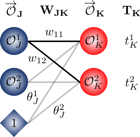
    Figure 1: NN showing the weights and outputs in vector form along with the target values for layer $K$

    Vectorising the Hidden Layer Deltas

    We need to vectorise:

    $$ \delta_{j} = \mathcal{O}_{i} \left( 1 - \mathcal{O}_{j} \right) \sum_{k \in K} \delta_{k} W_{jk} $$

    Let’s deal with the summation. We’re multipying each of the deltas $\delta_{k}$ in the output layer (or more generally, the subsequent layer could be another hidden layer) by the weight $w_{jk}$ that pulls them back to the node $j$ in the current layer before adding the results. For the first node in the hidden layer:

    $$ \sum_{k \in K} \delta_{k} W_{jk} = \delta_{k}^{1}w_{11} + \delta_{k}^{2}w_{12} + \delta_{k}^{3}w_{13} = \begin{pmatrix} w_{11} & w_{12} & w_{13} \end{pmatrix} \begin{pmatrix} \delta_{k}^{1} \\ \delta_{k}^{2} \\ \delta_{k}^{3}\end{pmatrix} $$

    Notice the weights? They pull the delta from each output layer node back to the first node of the hidden layer. In forward propagation, these we consider multiple nodes going out to a single node, rather than this way of receiving multiple nodes at a single node.

    Combine this summation with the multiplication by the activation function derivative:

    $$ \delta_{j}^{1} = \sigma^{\prime} \left( x_{j}^{1} \right) \begin{pmatrix} w_{11} & w_{12} & w_{13} \end{pmatrix} \begin{pmatrix} \delta_{k}^{1} \\ \delta_{k}^{2} \\ \delta_{k}^{3} \end{pmatrix} $$

    remembering that the input to the $\text{1}^\text{st}$ node in the layer $J$

    $$ x_{j}^{1} = \mathbf{W_{I1}}\mathbf{\vec{\mathcal{O}}_{I}} $$

    What about the $\text{2}^\text{nd}$ node in the hidden layer?

    $$ \delta_{j}^{2} = \sigma^{\prime} \left( x_{j}^{2} \right) \begin{pmatrix} w_{21} & w_{22} & w_{23} \end{pmatrix} \begin{pmatrix} \delta_{k}^{1} \\ \delta_{k}^{2} \\ \delta_{k}^{3} \end{pmatrix} $$

    This is looking familiar, hopefully we can be confident based upon what we’ve done before to say that:

    $$ \begin{pmatrix} \delta_{j}^{1} \\ \delta_{j}^{2} \end{pmatrix} = \begin{pmatrix} \sigma^{\prime} \left( x_{j}^{1} \right) \\ \sigma^{\prime} \left( x_{j}^{2} \right) \end{pmatrix} * \begin{pmatrix} w_{11} & w_{12} & w_{13} \\ w_{21} & w_{22} & w_{23} \end{pmatrix} \begin{pmatrix}\delta_{k}^{1} \\ \delta_{k}^{2} \\ \delta_{k}^{3} \end{pmatrix} $$

    We’ve seen a version of this weights matrix before when we did the forward propagation vectorisation. In this case though, look carefully - as we mentioned, the weights are not in the same places, in fact, the weight matrix has been transposed from the one we used in forward propagation. This makes sense because we’re going backwards through the network now! This is useful because it means there is very little extra calculation needed here - the matrix we need is already available from the forward pass, but just needs transposing. We can call the weights in back propagation here $ \mathbf{ W_{KJ}} $ as we’re pulling the deltas from $K$ to $J$.

    $$ \begin{align} \mathbf{W_{KJ}} &= \begin{pmatrix} w_{11} & w_{12} & \cdots & w_{1n} \\ w_{21} & w_{22} & \cdots & w_{23} \\ \vdots & \vdots & \ddots & \vdots \\ w_{(m+1)1} & w_{(m+1)2} & \cdots & w_{(m+1)n} \end{pmatrix} , \ \ \ \mathbf{W_{JK}} = \begin{pmatrix} w_{11} & w_{21} & \cdots & w_{(m+1)1} \\ w_{12} & w_{22} & \cdots & w_{(m+1)2} \\ \vdots & \vdots & \ddots & \vdots \\ w_{1n} & w_{2n} & \cdots & w_{(m+1)n} \\ \end{pmatrix} \\[0.5em] \mathbf{W_{KJ}} &= \mathbf{W^{\intercal}_{JK}} \end{align} $$
    And so, the vectorised equations for the output layer and hidden layer deltas are:
    $$ \begin{align} \mathbf{\vec{\delta}_{K}} &= \sigma^{\prime}\left( \mathbf{W_{JK}}\mathbf{\vec{\mathcal{O}}_{J}} \right) * \left( \mathbf{\vec{\mathcal{O}}_{K}} - \mathbf{T_{K}}\right) \\[0.5em] \mathbf{ \vec{ \delta }_{J}} &= \sigma^{\prime} \left( \mathbf{ W_{IJ} \mathcal{O}_{I} } \right) * \mathbf{ W^{\intercal}_{JK}} \mathbf{ \vec{\delta}_{K}} \end{align} $$

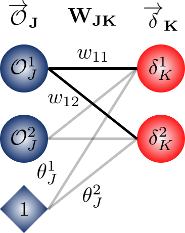
    Lets visualise what we’ve seen:

    Figure 2: The NN showing the delta vectors

    Vectorising the Update Equations

    Finally, now that we have the vectorised equations for the deltas (which required us to get the vectorised equations for the forward pass) we’re ready to get the update equations in vector form. Let’s recall the update equations

    $$ \begin{align} \Delta W &= -\eta \ \delta_{l} \ \mathcal{O}_{l-1} \\ \Delta\theta &= -\eta \ \delta_{l} \end{align} $$

    Ignoring the $-\eta$ for now, we need to get a vector form for $\delta_{l} \ \mathcal{O}_{l-1}$ in order to get the update to the weights. We have the matrix of weights:

    $$ \mathbf{W_{JK}} = \begin{pmatrix} w_{11} & w_{21} & w_{31} \\ w_{12} & w_{22} & w_{32} \\ \end{pmatrix} $$

    Suppose we are updating the weight $w_{21}$ in the matrix. We’re looking to find the product of the output from the second node in $J$ with the delta from the first node in $K$.

    $$ \Delta w_{21} = \delta_{K}^{1} \mathcal{O}_{J}^{2} $$

    Considering this example, we can write the matrix for the weight updates as:

    $$ \Delta \mathbf{W_{JK}} = \begin{pmatrix} \delta_{K}^{1} \mathcal{O}_{J}^{1} & \delta_{K}^{1} \mathcal{O}_{J}^{2} & \delta_{K}^{1} \mathcal{O}_{J}^{3} \\ \delta_{K}^{2} \mathcal{O}_{J}^{1} & \delta_{K}^{2} \mathcal{O}_{J}^{2} & \delta_{K}^{2} \mathcal{O}_{J}^{3} \end{pmatrix} = \begin{pmatrix} \delta_{K}^{1} \\ \delta_{K}^{2}\end{pmatrix} \begin{pmatrix} \mathcal{O}_{J}^{1} & \mathcal{O}_{J}^{2}& \mathcal{O}_{J}^{3} \end{pmatrix} $$

    Generalising this into vector notation and including the learning rate $\eta$, the update for the weights in layer $J$ is:

    $$ \Delta \mathbf{W_{JK}} = -\eta \mathbf{ \vec{ \delta }_{K}} \mathbf{ \vec { \mathcal{O} }_{J}} $$

    Similarly, we have the update to the bias term. If:

    $$ \Delta \vec{\theta} = -\eta \mathbf{ \vec{ \delta }_{K}} $$

    So the bias term is updated just by taking the deltas straight from the nodes in the subsequent layer (with the negative factor of learning rate).

    In summary, for back propagation, the equations we need in vector form are:
    $$ \begin{align} \mathbf{\vec{\delta}_{K}} &= \sigma^{\prime}\left( \mathbf{W_{JK}}\mathbf{\vec{\mathcal{O}}_{J}} \right) * \left( \mathbf{\vec{\mathcal{O}}_{K}} - \mathbf{T_{K}}\right) \\[0.5em] \mathbf{ \vec{ \delta }_{J}} &= \sigma^{\prime} \left( \mathbf{ W_{IJ} \mathcal{O}_{I} } \right) * \mathbf{ W^{\intercal}_{JK}} \mathbf{ \vec{\delta}_{K}} \end{align} $$
    $$ \begin{align} \mathbf{W_{JK}} + \Delta \mathbf{W_{JK}} &\rightarrow \mathbf{W_{JK}}, \ \ \ \Delta \mathbf{W_{JK}} = -\eta \mathbf{ \vec{ \delta }_{K}} \mathbf{ \vec { \mathcal{O} }_{J}} \\[0.5em] \vec{\theta} + \Delta \vec{\theta} &\rightarrow \vec{\theta}, \ \ \ \Delta \vec{\theta} = -\eta \mathbf{ \vec{ \delta }_{K}} \end{align} $$

    With $*$ representing an elementwise multiplication between the matrices.

    What's next?

    Although this kinds of mathematics can be tedious and sometimes hard to follow (and probably with numerous notation mistakes… please let me know if you find them!), it is necessary in order to write a quick, efficient NN. Our next step is to implement this setup in Python.

     
    comments powered by Disqus